7.3 Sampling Distributions
7.3: Sampling Distributions
7.3.1: What Is a Sampling Distribution?
The sampling distribution of a statistic is the distribution of the statistic for all possible samples from the same population of a given size.
Learning Objective
Recognize the characteristics of a sampling distribution
Key Takeaways
Key Points
- A critical part of inferential statistics involves determining how far sample statistics are likely to vary from each other and from the population parameter.
- The sampling distribution of a statistic is the distribution of that statistic, considered as a random variable, when derived from a random sample of size n.
- Sampling distributions allow analytical considerations to be based on the sampling distribution of a statistic rather than on the joint probability distribution of all the individual sample values.
- The sampling distribution depends on: the underlying distribution of the population, the statistic being considered, the sampling procedure employed, and the sample size used.
Key Terms
- inferential statistics
- A branch of mathematics that involves drawing conclusions about a population based on sample data drawn from it.
- sampling distribution
- The probability distribution of a given statistic based on a random sample.
Suppose you randomly sampled 10 women between the ages of 21 and 35 years from the population of women in Houston, Texas, and then computed the mean height of your sample. You would not expect your sample mean to be equal to the mean of all women in Houston. It might be somewhat lower or higher, but it would not equal the population mean exactly. Similarly, if you took a second sample of 10 women from the same population, you would not expect the mean of this second sample to equal the mean of the first sample.

Houston Skyline
Suppose you randomly sampled 10 people from the population of women in Houston, Texas between the ages of 21 and 35 years and computed the mean height of your sample. You would not expect your sample mean to be equal to the mean of all women in Houston.
Inferential statistics involves generalizing from a sample to a population. A critical part of inferential statistics involves determining how far sample statistics are likely to vary from each other and from the population parameter. These determinations are based on sampling distributions. The sampling distribution of a statistic is the distribution of that statistic, considered as a random variable, when derived from a random sample of size . It may be considered as the distribution of the statistic for all possible samples from the same population of a given size. Sampling distributions allow analytical considerations to be based on the sampling distribution of a statistic rather than on the joint probability distribution of all the individual sample values.
The sampling distribution depends on: the underlying distribution of the population, the statistic being considered, the sampling procedure employed, and the sample size used. For example, consider a normal population with mean and variance . Assume we repeatedly take samples of a given size from this population and calculate the arithmetic mean for each sample. This statistic is then called the sample mean. Each sample has its own average value, and the distribution of these averages is called the “sampling distribution of the sample mean. ” This distribution is normal since the underlying population is normal, although sampling distributions may also often be close to normal even when the population distribution is not.
An alternative to the sample mean is the sample median. When calculated from the same population, it has a different sampling distribution to that of the mean and is generally not normal (but it may be close for large sample sizes).
7.3.2: Properties of Sampling Distributions
Knowledge of the sampling distribution can be very useful in making inferences about the overall population.
Learning Objective
Describe the general properties of sampling distributions and the use of standard error in analyzing them
Key Takeaways
Key Points
- In practice, one will collect sample data and, from these data, estimate parameters of the population distribution.
- Knowing the degree to which means from different samples would differ from each other and from the population mean would give you a sense of how close your particular sample mean is likely to be to the population mean.
- The standard deviation of the sampling distribution of a statistic is referred to as the standard error of that quantity.
- If all the sample means were very close to the population mean, then the standard error of the mean would be small.
- On the other hand, if the sample means varied considerably, then the standard error of the mean would be large.
Key Terms
- inferential statistics
- A branch of mathematics that involves drawing conclusions about a population based on sample data drawn from it.
- sampling distribution
- The probability distribution of a given statistic based on a random sample.
Sampling Distributions and Inferential Statistics
Sampling distributions are important for inferential statistics. In practice, one will collect sample data and, from these data, estimate parameters of the population distribution. Thus, knowledge of the sampling distribution can be very useful in making inferences about the overall population.
For example, knowing the degree to which means from different samples differ from each other and from the population mean would give you a sense of how close your particular sample mean is likely to be to the population mean. Fortunately, this information is directly available from a sampling distribution. The most common measure of how much sample means differ from each other is the standard deviation of the sampling distribution of the mean. This standard deviation is called the standard error of the mean.
Standard Error
The standard deviation of the sampling distribution of a statistic is referred to as the standard error of that quantity. For the case where the statistic is the sample mean, and samples are uncorrelated, the standard error is:

Where S is the sample standard deviation and n is the size (number of items) in the sample. An important implication of this formula is that the sample size must be quadrupled (multiplied by 4) to achieve half the measurement error. When designing statistical studies where cost is a factor, this may have a role in understanding cost-benefit tradeoffs.
If all the sample means were very close to the population mean, then the standard error of the mean would be small. On the other hand, if the sample means varied considerably, then the standard error of the mean would be large. To be specific, assume your sample mean is 125 and you estimated that the standard error of the mean is 5. If you had a normal distribution, then it would be likely that your sample mean would be within 10 units of the population mean since most of a normal distribution is within two standard deviations of the mean.
More Properties of Sampling Distributions
- The overall shape of the distribution is symmetric and approximately normal.
- There are no outliers or other important deviations from the overall pattern.
- The center of the distribution is very close to the true population mean.
A statistical study can be said to be biased when one outcome is systematically favored over another. However, the study can be said to be unbiased if the mean of its sampling distribution is equal to the true value of the parameter being estimated.
Finally, the variability of a statistic is described by the spread of its sampling distribution. This spread is determined by the sampling design and the size of the sample. Larger samples give smaller spread. As long as the population is much larger than the sample (at least 10 times as large), the spread of the sampling distribution is approximately the same for any population size
7.3.3: Creating a Sampling Distribution
Learn to create a sampling distribution from a discrete set of data.
Learning Objective
Differentiate between a frequency distribution and a sampling distribution
Key Takeaways
Key Points
- Consider three pool balls, each with a number on it.
- Two of the balls are selected randomly (with replacement), and the average of their numbers is computed.
- The relative frequencies are equal to the frequencies divided by nine because there are nine possible outcomes.
- The distribution created from these relative frequencies is called the sampling distribution of the mean.
- As the number of samples approaches infinity, the frequency distribution will approach the sampling distribution.
Key Terms
- sampling distribution
- The probability distribution of a given statistic based on a random sample.
- frequency distribution
- a representation, either in a graphical or tabular format, which displays the number of observations within a given interval
We will illustrate the concept of sampling distributions with a simple example. Consider three pool balls, each with a number on it. Two of the balls are selected randomly (with replacement), and the average of their numbers is computed. All possible outcomes are shown below.
| Outcome | Ball 1 | Ball 2 | Mean |
|---|---|---|---|
| 1 | 1 | 1 | 1.0 |
| 2 | 1 | 2 | 1.5 |
| 3 | 1 | 3 | 2.0 |
| 4 | 2 | 1 | 1.5 |
| 5 | 2 | 2 | 2.0 |
| 6 | 2 | 3 | 2.5 |
| 7 | 3 | 1 | 2.0 |
| 8 | 3 | 2 | 2.5 |
| 9 | 3 | 3 | 3.0 |
Pool Ball Example 1
This table shows all the possible outcome of selecting two pool balls randomly from a population of three.
Notice that all the means are either 1.0, 1.5, 2.0, 2.5, or 3.0. The frequencies of these means are shown below. The relative frequencies are equal to the frequencies divided by nine because there are nine possible outcomes.
Pool Ball Example 2
This table shows the frequency of means for N=2.
The figure below shows a relative frequency distribution of the means. This distribution is also a probability distribution since the y-axis is the probability of obtaining a given mean from a sample of two balls in addition to being the relative frequency.
Relative Frequency Distribution
Relative frequency distribution of our pool ball example.
The distribution shown in the above figure is called the sampling distribution of the mean. Specifically, it is the sampling distribution of the mean for a sample size of 2 (). For this simple example, the distribution of pool balls and the sampling distribution are both discrete distributions. The pool balls have only the numbers 1, 2, and 3, and a sample mean can have one of only five possible values.
There is an alternative way of conceptualizing a sampling distribution that will be useful for more complex distributions. Imagine that two balls are sampled (with replacement), and the mean of the two balls is computed and recorded. This process is repeated for a second sample, a third sample, and eventually thousands of samples. After thousands of samples are taken and the mean is computed for each, a relative frequency distribution is drawn. The more samples, the closer the relative frequency distribution will come to the sampling distribution shown in the above figure. As the number of samples approaches infinity , the frequency distribution will approach the sampling distribution. This means that you can conceive of a sampling distribution as being a frequency distribution based on a very large number of samples. To be strictly correct, the sampling distribution only equals the frequency distribution exactly when there is an infinite number of samples.
7.3.4: Continuous Sampling Distributions
When we have a truly continuous distribution, it is not only impractical but actually impossible to enumerate all possible outcomes.
Learning Objective
Differentiate between discrete and continuous sampling distributions
Key Takeaways
Key Points
- In continuous distributions, the probability of obtaining any single value is zero.
- Therefore, these values are called probability densities rather than probabilities.
- A probability density function, or density of a continuous random variable, is a function that describes the relative likelihood for this random variable to take on a given value.
Key Term
- probability density function
- any function whose integral over a set gives the probability that a random variable has a value in that set
In the previous section, we created a sampling distribution out of a population consisting of three pool balls. This distribution was discrete, since there were a finite number of possible observations. Now we will consider sampling distributions when the population distribution is continuous.
What if we had a thousand pool balls with numbers ranging from 0.001 to 1.000 in equal steps? Note that although this distribution is not really continuous, it is close enough to be considered continuous for practical purposes. As before, we are interested in the distribution of the means we would get if we sampled two balls and computed the mean of these two. In the previous example, we started by computing the mean for each of the nine possible outcomes. This would get a bit tedious for our current example since there are 1,000,000 possible outcomes (1,000 for the first ball multiplied by 1,000 for the second.) Therefore, it is more convenient to use our second conceptualization of sampling distributions, which conceives of sampling distributions in terms of relative frequency distributions– specifically, the relative frequency distribution that would occur if samples of two balls were repeatedly taken and the mean of each sample computed.
Probability Density Function
When we have a truly continuous distribution, it is not only impractical but actually impossible to enumerate all possible outcomes. Moreover, in continuous distributions, the probability of obtaining any single value is zero. Therefore, these values are called probability densities rather than probabilities.
A probability density function, or density of a continuous random variable, is a function that describes the relative likelihood for this random variable to take on a given value. The probability for the random variable to fall within a particular region is given by the integral of this variable’s density over the region .

Probability Density Function
Boxplot and probability density function of a normal distribution N(0, 2).
7.3.5: Mean of All Sample Means (μ x)
The mean of the distribution of differences between sample means is equal to the difference between population means.
Learning Objectives
Discover that the mean of the distribution of differences between sample means is equal to the difference between population means
Key Takeaways
Key Points
- Statistical analysis are very often concerned with the difference between means.
- The mean of the sampling distribution of the mean is μM1−M2 = μ1−2.
- The variance sum law states that the variance of the sampling distribution of the difference between means is equal to the variance of the sampling distribution of the mean for Population 1 plus the variance of the sampling distribution of the mean for Population 2.
Key Term
- sampling distribution
- The probability distribution of a given statistic based on a random sample.
Statistical analyses are, very often, concerned with the difference between means. A typical example is an experiment designed to compare the mean of a control group with the mean of an experimental group. Inferential statistics used in the analysis of this type of experiment depend on the sampling distribution of the difference between means.
The sampling distribution of the difference between means can be thought of as the distribution that would result if we repeated the following three steps over and over again:
- Sample n1 scores from Population 1 and n2 scores from Population 2;
- Compute the means of the two samples ( M1 and M2);
- Compute the difference between means M1−M2. The distribution of the differences between means is the sampling distribution of the difference between means.
The mean of the sampling distribution of the mean is:
μM1−M2 = μ1−2,
which says that the mean of the distribution of differences between sample means is equal to the difference between population means. For example, say that mean test score of all 12-year olds in a population is 34 and the mean of 10-year olds is 25. If numerous samples were taken from each age group and the mean difference computed each time, the mean of these numerous differences between sample means would be 34 – 25 = 9.
The variance sum law states that the variance of the sampling distribution of the difference between means is equal to the variance of the sampling distribution of the mean for Population 1 plus the variance of the sampling distribution of the mean for Population 2. The formula for the variance of the sampling distribution of the difference between means is as follows:

Recall that the standard error of a sampling distribution is the standard deviation of the sampling distribution, which is the square root of the above variance.
Let’s look at an application of this formula to build a sampling distribution of the difference between means. Assume there are two species of green beings on Mars. The mean height of Species 1 is 32, while the mean height of Species 2 is 22. The variances of the two species are 60 and 70, respectively, and the heights of both species are normally distributed. You randomly sample 10 members of Species 1 and 14 members of Species 2.
The difference between means comes out to be 10, and the standard error comes out to be 3.317.
μM1−M2 = 32 – 22 = 10
Standard error equals the square root of (60 / 10) + (70 / 14) = 3.317.
The resulting sampling distribution as diagramed in , is normally distributed with a mean of 10 and a standard deviation of 3.317.
Sampling Distribution of the Difference Between Means
The distribution is normally distributed with a mean of 10 and a standard deviation of 3.317.
7.3.6: Shapes of Sampling Distributions
The overall shape of a sampling distribution is expected to be symmetric and approximately normal.
Learning Objective
Give examples of the various shapes a sampling distribution can take on
Key Takeaways
Key Points
- The concept of the shape of a distribution refers to the shape of a probability distribution.
- It most often arises in questions of finding an appropriate distribution to use to model the statistical properties of a population, given a sample from that population.
- A sampling distribution is assumed to have no outliers or other important deviations from the overall pattern.
- When calculated from the same population, the sample median has a different sampling distribution to that of the mean and is generally not normal; although, it may be close for large sample sizes.
Key Terms
- normal distribution
- A family of continuous probability distributions such that the probability density function is the normal (or Gaussian) function.
- skewed
- Biased or distorted (pertaining to statistics or information).
- Pareto Distribution
- The Pareto distribution, named after the Italian economist Vilfredo Pareto, is a power law probability distribution that is used in description of social, scientific, geophysical, actuarial, and many other types of observable phenomena.
- probability distribution
- A function of a discrete random variable yielding the probability that the variable will have a given value.
The “shape of a distribution” refers to the shape of a probability distribution. It most often arises in questions of finding an appropriate distribution to use in order to model the statistical properties of a population, given a sample from that population. The shape of a distribution will fall somewhere in a continuum where a flat distribution might be considered central; and where types of departure from this include:
- mounded (or unimodal)
- u-shaped
- j-shaped
- reverse-j-shaped
- multi-modal
The shape of a distribution is sometimes characterized by the behaviors of the tails (as in a long or short tail). For example, a flat distribution can be said either to have no tails or to have short tails. A normal distribution is usually regarded as having short tails, while a Pareto distribution has long tails. Even in the relatively simple case of a mounded distribution, the distribution may be skewed to the left or skewed to the right (with symmetric corresponding to no skew).
As previously mentioned, the overall shape of a sampling distribution is expected to be symmetric and approximately normal. This is due to the fact, or assumption, that there are no outliers or other important deviations from the overall pattern. This fact holds true when we repeatedly take samples of a given size from a population and calculate the arithmetic mean for each sample.
An alternative to the sample mean is the sample median. When calculated from the same population, it has a different sampling distribution to that of the mean and is generally not normal; although, it may be close for large sample sizes.

The Normal Distribution
Sample distributions, when the sampling statistic is the mean, are generally expected to display a normal distribution.
7.3.7: Sampling Distributions and the Central Limit Theorem
The central limit theorem for sample means states that as larger samples are drawn, the sample means form their own normal distribution.
Learning Objective
Illustrate that as the sample size gets larger, the sampling distribution approaches normality
Key Takeaways
Key Points
- The normal distribution has the same mean as the original distribution and a variance that equals the original variance divided by n, the sample size.
- is the number of values that are averaged together not the number of times the experiment is done.
- The usefulness of the theorem is that the sampling distribution approaches normality regardless of the shape of the population distribution.
Key Terms
- central limit theorem
- The theorem that states: If the sum of independent identically distributed random variables has a finite variance, then it will be (approximately) normally distributed.
- sampling distribution
- The probability distribution of a given statistic based on a random sample.
Example
Imagine rolling a large number of identical, unbiased dice. The distribution of the sum (or average) of the rolled numbers will be well approximated by a normal distribution. Since real-world quantities are often the balanced sum of many unobserved random events, the central limit theorem also provides a partial explanation for the prevalence of the normal probability distribution. It also justifies the approximation of large-sample statistics to the normal distribution in controlled experiments.
The central limit theorem states that, given certain conditions, the mean of a sufficiently large number of independent random variables, each with a well-defined mean and well-defined variance, will be (approximately) normally distributed. The central limit theorem has a number of variants. In its common form, the random variables must be identically distributed. In variants, convergence of the mean to the normal distribution also occurs for non-identical distributions, given that they comply with certain conditions.
The central limit theorem for sample means specifically says that if you keep drawing larger and larger samples (like rolling 1, 2, 5, and, finally, 10 dice) and calculating their means the sample means form their own normal distribution (the sampling distribution). The normal distribution has the same mean as the original distribution and a variance that equals the original variance divided by , the sample size. is the number of values that are averaged together not the number of times the experiment is done.
Classical Central Limit Theorem
Consider a sequence of independent and identically distributed random variables drawn from distributions of expected values given by and finite variances given by . Suppose we are interested in the sample average of these random variables. By the law of large numbers, the sample averages converge in probability and almost surely to the expected value as . The classical central limit theorem describes the size and the distributional form of the stochastic fluctuations around the deterministic number during this convergence. More precisely, it states that as gets larger, the distribution of the difference between the sample average and its limit approximates the normal distribution with mean 0 and variance . For large enough , the distribution of is close to the normal distribution with mean and variance

The upshot is that the sampling distribution of the mean approaches a normal distribution as , the sample size, increases. The usefulness of the theorem is that the sampling distribution approaches normality regardless of the shape of the population distribution.
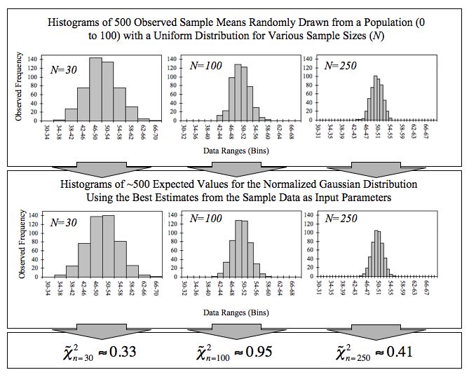
Empirical Central Limit Theorem
This figure demonstrates the central limit theorem. The sample means are generated using a random number generator, which draws numbers between 1 and 100 from a uniform probability distribution. It illustrates that increasing sample sizes result in the 500 measured sample means being more closely distributed about the population mean (50 in this case).
Attributions
- What Is a Sampling Distribution?
-
“David Lane, Introduction to Sampling Distributions. September 17, 2013.”
http://cnx.org/content/m11130/latest/.
OpenStax CNX
CC BY 3.0. -
“Sampling distribution.”
http://en.wikipedia.org/wiki/Sampling_distribution.
Wikipedia
CC BY-SA 3.0. -
“inferential statistics.”
http://en.wiktionary.org/wiki/inferential_statistics.
Wiktionary
CC BY-SA 3.0. -
“sampling distribution.”
http://en.wikipedia.org/wiki/sampling%20distribution.
Wikipedia
CC BY-SA 3.0. -
“All sizes | Houston Skyline | Flickr – Photo Sharing!.”
http://www.flickr.com/photos/mrbill/4803461/sizes/o/in/photostream/.
Flickr
CC BY.
- Properties of Sampling Distributions
-
“inferential statistics.”
http://en.wiktionary.org/wiki/inferential_statistics.
Wiktionary
CC BY-SA 3.0. -
“sampling distribution.”
http://en.wikipedia.org/wiki/sampling%20distribution.
Wikipedia
CC BY-SA 3.0. -
“Chapter 9-Sampling Distributions.”
http://mrschasesstatspage.wikispaces.com/Chapter+9-Sampling+Distributions.
mrschasesstatspage Wikispace
CC BY-SA 3.0. -
“David Lane, Introduction to Sampling Distributions. September 17, 2013.”
http://cnx.org/content/m11130/latest/.
OpenStax CNX
CC BY 3.0.
- Creating a Sampling Distribution
-
“sampling distribution.”
http://en.wikipedia.org/wiki/sampling%20distribution.
Wikipedia
CC BY-SA 3.0. -
“David Lane, Introduction to Sampling Distributions. September 17, 2013.”
http://cnx.org/content/m11130/latest/.
OpenStax CNX
CC BY 3.0. -
“David Lane, Introduction to Sampling Distributions. May 8, 2013.”
http://cnx.org/content/m11130/latest/.
OpenStax CNX
CC BY 3.0. -
“David Lane, Introduction to Sampling Distributions. May 8, 2013.”
http://cnx.org/content/m11130/latest/.
OpenStax CNX
CC BY 3.0. -
“David Lane, Introduction to Sampling Distributions. May 8, 2013.”
http://cnx.org/content/m11130/latest/.
OpenStax CNX
CC BY 3.0.
- Continuous Sampling Distributions
-
“Probability density function.”
http://en.wikipedia.org/wiki/Probability_density_function.
Wikipedia
CC BY-SA 3.0. -
“probability density function.”
http://en.wiktionary.org/wiki/probability_density_function.
Wiktionary
CC BY-SA 3.0. -
“David Lane, Introduction to Sampling Distributions. September 17, 2013.”
http://cnx.org/content/m11130/latest/.
OpenStax CNX
CC BY 3.0.
- Mean of All Sample Means (μ x)
-
“sampling distribution.”
http://en.wikipedia.org/wiki/sampling%20distribution.
Wikipedia
CC BY-SA 3.0. -
“David Lane, Sampling Distribution of Difference Between Means September 17, 2013.”
http://cnx.org/content/m11132/latest/.
OpenStax CNX
CC BY 3.0. -
“David Lane, Sampling Distribution of Difference Between Means May 10, 2013.”
http://cnx.org/content/m11132/latest/.
OpenStax CNX
CC BY 3.0.
- Shapes of Sampling Distributions
-
“Sampling distribution.”
http://en.wikipedia.org/wiki/Sampling_distribution.
Wikipedia
CC BY-SA 3.0. -
“Shape of the distribution.”
http://en.wikipedia.org/wiki/Shape_of_the_distribution.
Wikipedia
CC BY-SA 3.0. -
“probability distribution.”
http://en.wiktionary.org/wiki/probability_distribution.
Wiktionary
CC BY-SA 3.0. -
“Standard deviation diagram.”
http://commons.wikimedia.org/wiki/File:Standard_deviation_diagram.svg.
Wikimedia
CC BY.
- Sampling Distributions and the Central Limit Theorem
-
“Sampling distribution.”
http://en.wikipedia.org/wiki/Sampling_distribution.
Wikipedia
CC BY-SA 3.0. -
“Central limit theorem.”
http://en.wikipedia.org/wiki/Central_limit_theorem.
Wikipedia
CC BY-SA 3.0. -
“central limit theorem.”
http://en.wiktionary.org/wiki/central_limit_theorem.
Wiktionary
CC BY-SA 3.0. -
“sampling distribution.”
http://en.wikipedia.org/wiki/sampling%20distribution.
Wikipedia
CC BY-SA 3.0. -
“Susan Dean and Barbara Illowsky, Central Limit Theorem: Central Limit Theorem for Sample Means. September 17, 2013.”
http://cnx.org/content/m16947/latest/.
OpenStax CNX
CC BY 3.0. -
“Empirical CLT – Figure – 040711.”
http://commons.wikimedia.org/wiki/File:Empirical_CLT_-_Figure_-_040711.jpg.
Wikimedia
CC BY-SA.
