8.2 Probability Rules
8.2: Probability Rules
8.2.1: The Addition Rule
The addition rule states the probability of two events is the sum of the probability that either will happen minus the probability that both will happen.
Learning Objective
Calculate the probability of an event using the addition rule
Key Takeaways
Key Points
- The addition rule is:
- The last term has been accounted for twice, once in and once in , so it must be subtracted once so that it is not double-counted.
- If and are disjoint, then , so the formula becomes
Key Term
- probability
- The relative likelihood of an event happening.
Addition Law
The addition law of probability (sometimes referred to as the addition rule or sum rule), states that the probability that or will occur is the sum of the probabilities that will happen and that will happen, minus the probability that both and will happen. The addition rule is summarized by the formula:
Consider the following example. When drawing one card out of a deck of playing cards, what is the probability of getting heart or a face card (king, queen, or jack)? Let denote drawing a heart and denote drawing a face card. Since there are hearts and a total of face cards ( of each suit: spades, hearts, diamonds and clubs), but only face cards of hearts, we obtain:
Using the addition rule, we get:
The reason for subtracting the last term is that otherwise we would be counting the middle section twice (since and overlap).
Addition Rule for Disjoint Events
Suppose and are disjoint, their intersection is empty. Then the probability of their intersection is zero. In symbols: . The addition law then simplifies to:
The symbol represents the empty set, which indicates that in this case and do not have any elements in common (they do not overlap).
Example
Suppose a card is drawn from a deck of 52 playing cards: what is the probability of getting a king or a queen? Let represent the event that a king is drawn and represent the event that a queen is drawn. These two events are disjoint, since there are no kings that are also queens. Thus:


8.2.2: The Multiplication Rule
The multiplication rule states that the probability that A and B both occur is equal to the probability that B occurs times the conditional probability that A occurs given that B occurs.
Learning Objective
Apply the multiplication rule to calculate the probability of both A and B occurring
Key Takeaways
Key Points
- The multiplication rule can be written as: .
- We obtain the general multiplication rule by multiplying both sides of the definition of conditional probability by the denominator.
Key Term
- sample space
- The set of all possible outcomes of a game, experiment or other situation.
The Multiplication Rule
In probability theory, the Multiplication Rule states that the probability that and occur is equal to the probability that occurs times the conditional probability that occurs, given that we know has already occurred. This rule can be written:
Switching the role of and , we can also write the rule as:
We obtain the general multiplication rule by multiplying both sides of the definition of conditional probability by the denominator. That is, in the equation  , if we multiply both sides by , we obtain the Multiplication Rule.
The rule is useful when we know both and , or both and
Example
Suppose that we draw two cards out of a deck of cards and let be the event the the first card is an ace, and be the event that the second card is an ace, then:
And:
The denominator in the second equation is since we know a card has already been drawn. Therefore, there are left in total. We also know the first card was an ace, therefore:
Independent Event
Note that when and are independent, we have that , so the formula becomes , which we encountered in a previous section. As an example, consider the experiment of rolling a die and flipping a coin. The probability that we get a on the die and a tails on the coin is (, since the two events are independent.
8.2.3: Independence
To say that two events are independent means that the occurrence of one does not affect the probability of the other.
Learning Objective
Explain the concept of independence in relation to probability theory
Key Takeaways
Key Points
- Two events are independent if the following are true: ,, and .
- If any one of these conditions is true, then all of them are true.
- If events and are independent, then the chance of occurring does not affect the chance of occurring and vice versa.
Key Terms
- independence
- The occurrence of one event does not affect the probability of the occurrence of another.
- probability theory
- The mathematical study of probability (the likelihood of occurrence of random events in order to predict the behavior of defined systems).
Independent Events
In probability theory, to say that two events are independent means that the occurrence of one does not affect the probability that the other will occur. In other words, if events and are independent, then the chance of occurring does not affect the chance of occurring and vice versa. The concept of independence extends to dealing with collections of more than two events.

Independent Events
Selecting two cards from a deck by first selecting one, then replacing it in the deck before selecting a second is an example of independent events.
Two events are independent if any of the following are true:
To show that two events are independent, you must show only one of the conditions listed above. If any one of these conditions is true, then all of them are true.
Translating the symbols into words, the first two mathematical statements listed above say that the probability for the event with the condition is the same as the probability for the event without the condition. For independent events, the condition does not change the probability for the event. The third statement says that the probability of both independent events and occurring is the same as the probability of occurring, multiplied by the probability of occurring.
As an example, imagine you select two cards consecutively from a complete deck of playing cards. The two selections are not independent. The result of the first selection changes the remaining deck and affects the probabilities for the second selection. This is referred to as selecting “without replacement” because the first card has not been replaced into the deck before the second card is selected.
However, suppose you were to select two cards “with replacement” by returning your first card to the deck and shuffling the deck before selecting the second card. Because the deck of cards is complete for both selections, the first selection does not affect the probability of the second selection. When selecting cards with replacement, the selections are independent.
Consider a fair die role, which provides another example of independent events. If a person roles two die, the outcome of the first roll does not change the probability for the outcome of the second roll.
Example
Two friends are playing billiards, and decide to flip a coin to determine who will play first during each round. For the first two rounds, the coin lands on heads. They decide to play a third round, and flip the coin again. What is the probability that the coin will land on heads again?
First, note that each coin flip is an independent event. The side that a coin lands on does not depend on what occurred previously.
For any coin flip, there is a 1/2 chance that the coin will land on heads. Thus, the probability that the coin will land on heads during the third round is 1/2.
Example
When flipping a coin, what is the probability of getting tails 5 times in a row?
Recall that each coin flip is independent, and the probability of getting tails is 1/2 for any flip. Also recall that the following statement holds true for any two independent events A and B:
Finally, the concept of independence extends to collections of more than 2 events.
Therefore, the probability of getting tails 4 times in a row is:

8.2.4: Counting Rules and Techniques
Combinatorics is a branch of mathematics concerning the study of finite or countable discrete structures.
Learning Objective
Describe the different rules and properties for combinatorics
Key Takeaways
Key Points
- The rule of sum (addition rule), rule of product (multiplication rule), and inclusion-exclusion principle are often used for enumerative purposes.
- Bijective proofs are utilized to demonstrate that two sets have the same number of elements.
- Double counting is a technique used to demonstrate that two expressions are equal. The pigeonhole principle often ascertains the existence of something or is used to determine the minimum or maximum number of something in a discrete context.
- Generating functions and recurrence relations are powerful tools that can be used to manipulate sequences, and can describe if not resolve many combinatorial situations.
- Double counting is a technique used to demonstrate that two expressions are equal.
Key Terms
- polynomial
- An expression consisting of a sum of a finite number of terms: each term being the product of a constant coefficient and one or more variables raised to a non-negative integer power.
- combinatorics
- A branch of mathematics that studies (usually finite) collections of objects that satisfy specified criteria.
Combinatorics is a branch of mathematics concerning the study of finite or countable discrete structures. Combinatorial techniques are applicable to many areas of mathematics, and a knowledge of combinatorics is necessary to build a solid command of statistics. It involves the enumeration, combination, and permutation of sets of elements and the mathematical relations that characterize their properties.
Aspects of combinatorics include: counting the structures of a given kind and size, deciding when certain criteria can be met, and constructing and analyzing objects meeting the criteria. Aspects also include finding “largest,” “smallest,” or “optimal” objects, studying combinatorial structures arising in an algebraic context, or applying algebraic techniques to combinatorial problems.
Combinatorial Rules and Techniques
Several useful combinatorial rules or combinatorial principles are commonly recognized and used. Each of these principles is used for a specific purpose. The rule of sum (addition rule), rule of product (multiplication rule), and inclusion-exclusion principle are often used for enumerative purposes. Bijective proofs are utilized to demonstrate that two sets have the same number of elements. Double counting is a method of showing that two expressions are equal. The pigeonhole principle often ascertains the existence of something or is used to determine the minimum or maximum number of something in a discrete context. Generating functions and recurrence relations are powerful tools that can be used to manipulate sequences, and can describe if not resolve many combinatorial situations. Each of these techniques is described in greater detail below.
Rule of Sum
The rule of sum is an intuitive principle stating that if there are possible ways to do something, and possible ways to do another thing, and the two things can’t both be done, then there are total possible ways to do one of the things. More formally, the sum of the sizes of two disjoint sets is equal to the size of the union of these sets.
Rule of Product
The rule of product is another intuitive principle stating that if there are ways to do something and ways to do another thing, then there are ways to do both things.
Inclusion-Exclusion Principle
The inclusion-exclusion principle is a counting technique that is used to obtain the number of elements in a union of multiple sets. This counting method ensures that elements that are present in more than one set in the union are not counted more than once. It considers the size of each set and the size of the intersections of the sets. The smallest example is when there are two sets: the number of elements in the union of and is equal to the sum of the number of elements in and , minus the number of elements in their intersection. See the diagram below for an example with three sets.
Bijective Proof
A bijective proof is a proof technique that finds a bijective function between two finite sets and , which proves that they have the same number of elements, . A bijective function is one in which there is a one-to-one correspondence between the elements of two sets. In other words, each element in set is paired with exactly one element in set . This technique is useful if we wish to know the size of , but can find no direct way of counting its elements. If is more easily countable, establishing a bijection from to solves the problem.
Double Counting
Double counting is a combinatorial proof technique for showing that two expressions are equal. This is done by demonstrating that the two expressions are two different ways of counting the size of one set. In this technique, a finite set is described from two perspectives, leading to two distinct expressions for the size of the set. Since both expressions equal the size of the same set, they equal each other.
Pigeonhole Principle
The pigeonhole principle states that if items are each put into one of boxes, where , then at least one of the boxes contains more than one item. This principle allows one to demonstrate the existence of some element in a set with some specific properties. For example, consider a set of three gloves. In such a set, there must be either two left gloves or two right gloves (or three of left or right). This is an application of the pigeonhole principle that yields information about the properties of the gloves in the set.
Generating Function
Generating functions can be thought of as polynomials with infinitely many terms whose coefficients correspond to the terms of a sequence. The (ordinary) generating function of a sequence is given by:

whose coefficients give the sequence .
Recurrence Relation
A recurrence relation defines each term of a sequence in terms of the preceding terms. In other words, once one or more initial terms are given, each of the following terms of the sequence is a function of the preceding terms.
The Fibonacci sequence is one example of a recurrence relation. Each term of the Fibonacci sequence is given by , with initial values and . Thus, the sequence of Fibonacci numbers begins:
8.2.5: Bayes’ Rule
Bayes’ rule expresses how a subjective degree of belief should rationally change to account for evidence.
Learning Objective
Explain the importance of Bayes’s theorem in mathematical manipulation of conditional probabilities
Key Takeaways
Key Points
- Bayes’ rule relates the odds of event to event , before (prior to) and after (posterior to) conditioning on another event .
- More specifically, given events , , and , Bayes’ rule states that the conditional odds of given are equal to the marginal odds if multiplied by the Bayes’ factor.
- Bayes’ rule shows how one’s judgement on whether or is true should be updated based on observing the evidence.
- Bayesian inference is a method of inference in which Bayes’ rule is used to update the probability estimate for a hypothesis as additional evidence is learned.
Key Term
- Bayes’ factor
- The ratio of the conditional probabilities of the event $B$ given that $A_1$ is the case or that $A_2$ is the case, respectively.
In probability theory and statistics, Bayes’ theorem (or Bayes’ rule ) is a result that is of importance in the mathematical manipulation of conditional probabilities. It is a result that derives from the more basic axioms of probability. When applied, the probabilities involved in Bayes’ theorem may have any of a number of probability interpretations. In one of these interpretations, the theorem is used directly as part of a particular approach to statistical inference. In particular, with the Bayesian interpretation of probability, the theorem expresses how a subjective degree of belief should rationally change to account for evidence. This is known as Bayesian inference, which is fundamental to Bayesian statistics.
Bayes’ rule relates the odds of event to event , before (prior to) and after (posterior to) conditioning on another event . The odds on to event is simply the ratio of the probabilities of the two events. The relationship is expressed in terms of the likelihood ratio, or Bayes’ factor. By definition, this is the ratio of the conditional probabilities of the event given that is the case or that is the case, respectively. The rule simply states:
Posterior odds equals prior odds times Bayes’ factor.
More specifically, given events , and , Bayes’ rule states that the conditional odds of given are equal to the marginal odds multiplied by the Bayes factor or likelihood ratio. This is shown in the following formulas:
Where the likelihood ratio is the ratio of the conditional probabilities of the event given that is the case or that is the case, respectively:
Bayes’ rule is widely used in statistics, science and engineering, such as in: model selection, probabilistic expert systems based on Bayes’ networks, statistical proof in legal proceedings, email spam filters, etc. Bayes’ rule tells us how unconditional and conditional probabilities are related whether we work with a frequentist or a Bayesian interpretation of probability. Under the Bayesian interpretation it is frequently applied in the situation where and are competing hypotheses, and is some observed evidence. The rule shows how one’s judgement on whether or is true should be updated on observing the evidence.
Bayesian Inference
Bayesian inference is a method of inference in which Bayes’ rule is used to update the probability estimate for a hypothesis as additional evidence is learned. Bayesian updating is an important technique throughout statistics, and especially in mathematical statistics. Bayesian updating is especially important in the dynamic analysis of a sequence of data. Bayesian inference has found application in a range of fields including science, engineering, philosophy, medicine, and law.
Informal Definition
Rationally, Bayes’ rule makes a great deal of sense. If the evidence does not match up with a hypothesis, one should reject the hypothesis. But if a hypothesis is extremely unlikely a priori, one should also reject it, even if the evidence does appear to match up.
For example, imagine that we have various hypotheses about the nature of a newborn baby of a friend, including:
- H1: The baby is a brown-haired boy.
- H2: The baby is a blond-haired girl.
- H3: The baby is a dog.
Then, consider two scenarios:
- We’re presented with evidence in the form of a picture of a blond-haired baby girl. We find this evidence supports and opposes and .
- We’re presented with evidence in the form of a picture of a baby dog. Although this evidence, treated in isolation, supports , my prior belief in this hypothesis (that a human can give birth to a dog) is extremely small. Therefore, the posterior probability is nevertheless small.
The critical point about Bayesian inference, then, is that it provides a principled way of combining new evidence with prior beliefs, through the application of Bayes’ rule. Furthermore, Bayes’ rule can be applied iteratively. After observing some evidence, the resulting posterior probability can then be treated as a prior probability, and a new posterior probability computed from new evidence. This allows for Bayesian principles to be applied to various kinds of evidence, whether viewed all at once or over time. This procedure is termed Bayesian updating.
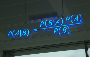
Bayes’ Theorem
A blue neon sign at the Autonomy Corporation in Cambridge, showing the simple statement of Bayes’ theorem.
8.2.6: The Collins Case
The People of the State of California v. Collins was a 1968 jury trial in California that made notorious forensic use of statistics and probability.
Learning Objective
Argue what causes prosecutor’s fallacy
Key Takeaways
Key Points
- Bystanders to a robbery in Los Angeles testified that the perpetrators had been a black male, with a beard and moustache, and a caucasian female with blonde hair tied in a ponytail. They had escaped in a yellow motor car.
- A witness of the prosecution, an instructor in mathematics, explained the multiplication rule to the jury, but failed to give weight to independence, or the difference between conditional and unconditional probabilities.
- The Collins case is a prime example of a phenomenon known as the prosecutor’s fallacy.
Key Terms
- multiplication rule
- The probability that A and B occur is equal to the probability that A occurs times the probability that B occurs, given that we know A has already occurred.
- prosecutor’s fallacy
- A fallacy of statistical reasoning when used as an argument in legal proceedings.
The People of the State of California v. Collins was a 1968 jury trial in California. It made notorious forensic use of statistics and probability. Bystanders to a robbery in Los Angeles testified that the perpetrators had been a black male, with a beard and moustache, and a caucasian female with blonde hair tied in a ponytail. They had escaped in a yellow motor car.
The prosecutor called upon for testimony an instructor in mathematics from a local state college. The instructor explained the multiplication rule to the jury, but failed to give weight to independence, or the difference between conditional and unconditional probabilities. The prosecutor then suggested that the jury would be safe in estimating the following probabilities:
- Black man with beard: 1 in 10
- Man with moustache: 1 in 4
- White woman with pony tail: 1 in 10
- White woman with blonde hair: 1 in 3
- Yellow motor car: 1 in 10
- Interracial couple in car: 1 in 1000
These probabilities, when considered together, result in a 1 in 12,000,000 chance that any other couple with similar characteristics had committed the crime – according to the prosecutor, that is. The jury returned a verdict of guilty.
As seen in , upon appeal, the Supreme Court of California set aside the conviction, criticizing the statistical reasoning and disallowing the way the decision was put to the jury. In their judgment, the justices observed that mathematics:

The Collins Case
The Collins case is a classic example of the prosecutor’s fallacy. The guilty verdict was reversed upon appeal to the Supreme Court of California in 1968.
… while assisting the trier of fact in the search of truth, must not cast a spell over him.
Prosecutor’s Fallacy
The Collins’ case is a prime example of a phenomenon known as the prosecutor’s fallacy—a fallacy of statistical reasoning when used as an argument in legal proceedings. At its heart, the fallacy involves assuming that the prior probability of a random match is equal to the probability that the defendant is innocent. For example, if a perpetrator is known to have the same blood type as a defendant (and 10% of the population share that blood type), to argue solely on that basis that the probability of the defendant being guilty is 90% makes the prosecutors’s fallacy (in a very simple form).
The basic fallacy results from misunderstanding conditional probability, and neglecting the prior odds of a defendant being guilty before that evidence was introduced. When a prosecutor has collected some evidence (for instance, a DNA match) and has an expert testify that the probability of finding this evidence if the accused were innocent is tiny, the fallacy occurs if it is concluded that the probability of the accused being innocent must be comparably tiny. If the DNA match is used to confirm guilt that is otherwise suspected, then it is indeed strong evidence. However, if the DNA evidence is the sole evidence against the accused, and the accused was picked out of a large database of DNA profiles, then the odds of the match being made at random may be reduced. Therefore, it is less damaging to the defendant. The odds in this scenario do not relate to the odds of being guilty; they relate to the odds of being picked at random.
Attributions
- The Addition Rule
- The Multiplication Rule
- Independence
-
“Independence (probability theory).”
http://en.wikipedia.org/wiki/Independence_(probability_theory).
Wikipedia
CC BY-SA 3.0. -
“Roberta Bloom, Probability Topics: Independent & Mutually Exclusive Events (modified R. Bloom). September 17, 2013.”
http://cnx.org/content/m18868/latest/.
OpenStax CNX
CC BY 3.0. -
“All sizes | Ace of Spades Card Deck Trick Magic Macro 10-19-09 2 | Flickr – Photo Sharing!.”
http://www.flickr.com/photos/stevendepolo/4028160820/sizes/o/in/photostream/.
Flickr
CC BY.
- Counting Rules and Techniques
-
“Double counting (proof technique).”
http://en.wikipedia.org/wiki/Double_counting_(proof_technique).
Wikipedia
CC BY-SA 3.0. -
“Inclusion-exclusion principle.”
https://en.wikipedia.org/wiki/Inclusion%E2%80%93exclusion_principle.
Wikipedia
CC BY-SA 3.0. -
“Combinatorial principles.”
http://en.wikipedia.org/wiki/Combinatorial_principles.
Wikipedia
CC BY-SA 3.0.
- Bayes’ Rule
-
“Bayes’ Theorem MMB 01.”
http://commons.wikimedia.org/wiki/File:Bayes’_Theorem_MMB_01.jpg.
Wikimedia
CC BY-SA.
- The Collins Case
-
“prosecutor’s fallacy.”
http://en.wikipedia.org/wiki/prosecutor’s%20fallacy.
Wikipedia
CC BY-SA 3.0.
