5.3 The Law of Averages
5.3: The Law of Averages
5.3.1: What Does the Law of Averages Say?
The law of averages is a lay term used to express a belief that outcomes of a random event will “even out” within a small sample.
Learning Objectives
Evaluate the law of averages and distinguish it from the law of large numbers.
Key Takeaways
Key Points
- The law of averages typically assumes that unnatural short-term “balance” must occur. This can also be known as “Gambler’s Fallacy” and is not a real mathematical principle.
- Some people mix up the law of averages with the law of large numbers, which is a real theorem that states that the average of the results obtained from a large number of trials should be close to the expected value, and will tend to become closer as more trials are performed.
- The law of large numbers is important because it “guarantees” stable long-term results for the averages of random events. It does not guarantee what will happen with a small number of events.
Key Term
- expected value
- of a discrete random variable, the sum of the probability of each possible outcome of the experiment multiplied by the value itself
The Law of Averages
The law of averages is a lay term used to express a belief that outcomes of a random event will “even out” within a small sample. As invoked in everyday life, the “law” usually reflects bad statistics or wishful thinking rather than any mathematical principle. While there is a real theorem that a random variable will reflect its underlying probability over a very large sample (the law of large numbers), the law of averages typically assumes that unnatural short-term “balance” must occur.
The law of averages is sometimes known as “Gambler’s Fallacy. ” It evokes the idea that an event is “due” to happen. For example, “The roulette wheel has landed on red in three consecutive spins. The law of averages says it’s due to land on black! ” Of course, the wheel has no memory and its probabilities do not change according to past results. So even if the wheel has landed on red in ten consecutive spins, the probability that the next spin will be black is still 48.6% (assuming a fair European wheel with only one green zero: it would be exactly 50% if there were no green zero and the wheel were fair, and 47.4% for a fair American wheel with one green “0” and one green “00”). (In fact, if the wheel has landed on red in ten consecutive spins, that is strong evidence that the wheel is not fair – that it is biased toward red. Thus, the wise course on the eleventh spin would be to bet on red, not on black: exactly the opposite of the layman’s analysis.) Similarly, there is no statistical basis for the belief that lottery numbers which haven’t appeared recently are due to appear soon.
The Law of Large Numbers
Some people interchange the law of averages with the law of large numbers, but they are different. The law of averages is not a mathematical principle, whereas the law of large numbers is. In probability theory, the law of large numbers is a theorem that describes the result of performing the same experiment a large number of times. According to the law, the average of the results obtained from a large number of trials should be close to the expected value, and will tend to become closer as more trials are performed.
The law of large numbers is important because it “guarantees” stable long-term results for the averages of random events. For example, while a casino may lose money in a single spin of the roulette wheel, its earnings will tend towards a predictable percentage over a large number of spins. Any winning streak by a player will eventually be overcome by the parameters of the game. It is important to remember that the law of large numbers only applies (as the name indicates) when a large number of observations are considered. There is no principle that a small number of observations will coincide with the expected value or that a streak of one value will immediately be “balanced” by the others.
Another good example comes from the expected value of rolling a six-sided die. A single roll produces one of the numbers 1, 2, 3, 4, 5, or 6, each with an equal probability (
) of occurring. The expected value of a roll is 3.5, which comes from the following equation:
According to the law of large numbers, if a large number of six-sided dice are rolled, the average of their values (sometimes called the sample mean ) is likely to be close to 3.5, with the accuracy increasing as more dice are rolled. However, in a small number of rolls, just because ten 6’s are rolled in a row, it doesn’t mean a 1 is more likely the next roll. Each individual outcome still has a probability of
.

The Law of Large Numbers: This shows a graph illustrating the law of large numbers using a particular run of rolls of a single die. As the number of rolls in this run increases, the average of the values of all the results approaches 3.5. While different runs would show a different shape over a small number of throws (at the left), over a large number of rolls (to the right) they would be extremely similar.
5.3.2: Chance Processes
A stochastic process is a collection of random variables that is often used to represent the evolution of some random value over time.
Learning Objective
Summarize the stochastic process and state its relationship to random walks.
Key Takeaways
Key Points
- One approach to stochastic processes treats them as functions of one or several deterministic arguments (inputs, in most cases regarded as time) whose values (outputs) are random variables.
- Random variables are non-deterministic (single) quantities which have certain probability distributions.
- Although the random values of a stochastic process at different times may be independent random variables, in most commonly considered situations they exhibit complicated statistical correlations.
- The law of a stochastic process is the measure that the process induces on the collection of functions from the index set into the state space.
- A random walk is a mathematical formalization of a path that consists of a succession of random steps.
Key Terms
- random variable
- a quantity whose value is random and to which a probability distribution is assigned, such as the possible outcome of a roll of a die
- random walk
- a stochastic path consisting of a series of sequential movements, the direction (and sometime length) of which is chosen at random
- stochastic
- random; randomly determined
Example
Familiar examples of processes modeled as stochastic time series include stock market and exchange rate fluctuations; signals such as speech, audio and video; medical data such as a patient’s EKG, EEG, blood pressure or temperature; and random movement such as Brownian motion or random walks.
Chance = Stochastic
In probability theory, a stochastic process–sometimes called a random process– is a collection of random variables that is often used to represent the evolution of some random value, or system, over time. It is the probabilistic counterpart to a deterministic process (or deterministic system). Instead of describing a process which can only evolve in one way (as in the case, for example, of solutions of an ordinary differential equation), in a stochastic or random process there is some indeterminacy. Even if the initial condition (or starting point) is known, there are several (often infinitely many) directions in which the process may evolve.
In the simple case of discrete time, a stochastic process amounts to a sequence of random variables known as a time series–for example, a Markov chain. Another basic type of a stochastic process is a random field, whose domain is a region of space. In other words, a stochastic process is a random function whose arguments are drawn from a range of continuously changing values.
One approach to stochastic processes treats them as functions of one or several deterministic arguments (inputs, in most cases regarded as time) whose values (outputs) are random variables. Random variables are non-deterministic (single) quantities which have certain probability distributions. Random variables corresponding to various times (or points, in the case of random fields) may be completely different. Although the random values of a stochastic process at different times may be independent random variables, in most commonly considered situations they exhibit complicated statistical correlations.
Familiar examples of processes modeled as stochastic time series include stock market and exchange rate fluctuations; signals such as speech, audio, and video; medical data such as a patient’s EKG, EEG, blood pressure, or temperature; and random movement such as Brownian motion or random walks.
Law of a Stochastic Process
The law of a stochastic process is the measure that the process induces on the collection of functions from the index set into the state space. The law encodes a lot of information about the process. In the case of a random walk, for example, the law is the probability distribution of the possible trajectories of the walk.
A random walk is a mathematical formalization of a path that consists of a succession of random steps. For example, the path traced by a molecule as it travels in a liquid or a gas, the search path of a foraging animal, the price of a fluctuating stock, and the financial status of a gambler can all be modeled as random walks, although they may not be truly random in reality. Random walks explain the observed behaviors of processes in such fields as ecology, economics, psychology, computer science, physics, chemistry, biology and, of course, statistics. Thus, the random walk serves as a fundamental model for recorded stochastic activity.

Random Walk
Example of eight random walks in one dimension starting at 0. The plot shows the current position on the line (vertical axis) versus the time steps (horizontal axis).
5.3.3: The Sum of Draws
The sum of draws is the process of drawing randomly, with replacement, from a set of data and adding up the results.
Learning Objective
Describe how chance variation affects sums of draws.
Key Takeaways
Key Points
- By drawing from a set of data with replacement, we are able to draw over and over again under the same conditions.
- The sum of draws is subject to a force known as chance variation.
- The sum of draws can be illustrated in practice through a game of Monopoly. A player rolls a pair of dice, adds the two numbers on the die, and moves his or her piece that many squares.
Key Term
- chance variation
- the presence of chance in determining the variation in experimental results
The sum of draws can be illustrated by the following process. Imagine there is a box of tickets, each having a number 1, 2, 3, 4, 5, or 6 written on it.
The sum of draws can be represented by a process in which tickets are drawn at random from the box, with the ticket being replaced to the box after each draw. Then, the numbers on these tickets are added up. By replacing the tickets after each draw, you are able to draw over and over under the same conditions.
Say you draw twice from the box at random with replacement. To find the sum of draws, you simply add the first number you drew to the second number you drew. For instance, if first you draw a 4 and second you draw a 6, your sum of draws would be . You could also first draw a 4 and then draw 4 again. In this case your sum of draws would be . Your sum of draws is, therefore, subject to a force known as chance variation.
This example can be seen in practical terms when imagining a turn of Monopoly. A player rolls a pair of dice, adds the two numbers on the die, and moves his or her piece that many squares. Rolling a die is the same as drawing a ticket from a box containing six options.
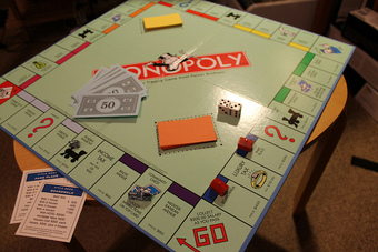
Sum of Draws In Practice
Rolling a die is the same as drawing a ticket from a box containing six options.
To better see the affects of chance variation, let us take 25 draws from the box. These draws result in the following values:
3 2 4 6 3 3 5 4 4 1 3 6 4 1 3 4 1 5 5 5 2 2 2 5 6
The sum of these 25 draws is 89. Obviously this sum would have been different had the draws been different.
5.3.4: Making a Box Model
A box plot (also called a box-and-whisker diagram) is a simple visual representation of key features of a univariate sample.
Learning Objectives
Produce a box plot that is representative of a data set.
Key Takeaways
Key Points
- Our ultimate goal in statistics is not to summarize the data, it is to fully understand their complex relationships.
- A well designed statistical graphic helps us explore, and perhaps understand, these relationships.
- A common extension of the box model is the ‘box-and-whisker’ plot, which adds vertical lines extending from the top and bottom of the plot to, for example, the maximum and minimum values.
Key Terms
- regression
- An analytic method to measure the association of one or more independent variables with a dependent variable.
- box-and-whisker plot
- a convenient way of graphically depicting groups of numerical data through their quartiles
A single statistic tells only part of a dataset’s story. The mean is one perspective; the median yet another. When we explore relationships between multiple variables, even more statistics arise, such as the coefficient estimates in a regression model or the Cochran-Maentel-Haenszel test statistic in partial contingency tables. A multitude of statistics are available to summarize and test data.
Our ultimate goal in statistics is not to summarize the data, it is to fully understand their complex relationships. A well designed statistical graphic helps us explore, and perhaps understand, these relationships. A box plot (also called a box and whisker diagram) is a simple visual representation of key features of a univariate sample.
The box lies on a vertical axis in the range of the sample. Typically, a top to the box is placed at the first quartile, the bottom at the third quartile. The width of the box is arbitrary, as there is no x-axis. In between the top and bottom of the box is some representation of central tendency. A common version is to place a horizontal line at the median, dividing the box into two. Additionally, a star or asterisk is placed at the mean value, centered in the box in the horizontal direction.
Another common extension of the box model is the ‘box-and-whisker’ plot , which adds vertical lines extending from the top and bottom of the plot to, for example, the maximum and minimum values. Alternatively, the whiskers could extend to the 2.5 and 97.5 percentiles. Finally, it is common in the box-and-whisker plot to show outliers (however defined) with asterisks at the individual values beyond the ends of the whiskers.

Box-and-Whisker Plot
Box plot of data from the Michelson-Morley Experiment, which attempted to detect the relative motion of matter through the stationary luminiferous aether.
Attributions
- What Does the Law of Averages Say?
- Chance Processes
-
“Law (stochastic processes).”
http://en.wikipedia.org/wiki/Law_(stochastic_processes).
Wikipedia
CC BY-SA 3.0. -
“Random Walk example.”
http://commons.wikimedia.org/wiki/File:Random_Walk_example.svg.
Wikimedia
GNU FDL 1.2.
- The Sum of Draws
-
“Sampling (statistics).”
http://en.wikipedia.org/wiki/Sampling_(statistics).
Wikipedia
CC BY-SA 3.0. -
“All sizes | Monopoly | Flickr – Photo Sharing!.”
http://www.flickr.com/photos/elpadawan/8480394254/sizes/z/in/photostream/.
Flickr
CC BY-SA.
- Making a Box Model
-
“box-and-whisker plot.”
http://en.wikipedia.org/wiki/box-and-whisker%20plot.
Wikipedia
CC BY-SA 3.0. -
“Statistics/Displaying Data/Box Plots.”
http://en.wikibooks.org/wiki/Statistics/Displaying_Data/Box_Plots.
Wikibooks
CC BY-SA 3.0. -
“Statistics/Displaying Data.”
http://en.wikibooks.org/wiki/Statistics/Displaying_Data.
Wikibooks
CC BY-SA 3.0. -
“Michelsonmorley-boxplot.”
http://commons.wikimedia.org/wiki/File:Michelsonmorley-boxplot.svg.
Wikimedia
Public domain. -
“Michelsonmorley-boxplot.”
http://en.wikipedia.org/wiki/File:Michelsonmorley-boxplot.svg.
Wikipedia
Public domain.
