7.4 Errors in Sampling
7.4: Errors in Sampling
7.4.1: Expected Value and Standard Error
Expected value and standard error can provide useful information about the data recorded in an experiment.
Learning Objective
Solve for the standard error of a sum and the expected value of a random variable
Key Takeaways
Key Points
- The expected value (or expectation, mathematical expectation, EV, mean, or first moment) of a random variable is the weighted average of all possible values that this random variable can take on.
- The expected value may be intuitively understood by the law of large numbers: the expected value, when it exists, is almost surely the limit of the sample mean as sample size grows to infinity.
- The standard error is the standard deviation of the sampling distribution of a statistic.
- The standard error of the sum represents how much one can expect the actual value of a repeated experiment to vary from the expected value of that experiment.
Key Terms
- standard deviation
- a measure of how spread out data values are around the mean, defined as the square root of the variance
- continuous random variable
- obtained from data that can take infinitely many values
- discrete random variable
- obtained by counting values for which there are no in-between values, such as the integers 0, 1, 2, ….
Expected Value
In probability theory, the expected value (or expectation, mathematical expectation, EV, mean, or first moment) of a random variable is the weighted average of all possible values that this random variable can take on. The weights used in computing this average are probabilities in the case of a discrete random variable, or values of a probability density function in the case of a continuous random variable.
The expected value may be intuitively understood by the law of large numbers: the expected value, when it exists, is almost surely the limit of the sample mean as sample size grows to infinity. More informally, it can be interpreted as the long-run average of the results of many independent repetitions of an experiment (e.g. a dice roll). The value may not be expected in the ordinary sense—the “expected value” itself may be unlikely or even impossible (such as having 2.5 children), as is also the case with the sample mean.
The expected value of a random variable can be calculated by summing together all the possible values with their weights (probabilities):
![E[X]=X_1P_1+X_2P_2+...+X_kP_k](https://open.ocolearnok.org/app/uploads/quicklatex/quicklatex.com-71bb4def706886486f4ccd78a9957fad_l3.png "Rendered by QuickLaTeX.com")
where represents a possible value and represents the probability of that possible value.
Standard Error
The standard error is the standard deviation of the sampling distribution of a statistic. For example, the sample mean s the usual estimator of a population mean. However, different samples drawn from that same population would in general have different values of the sample mean. The standard error of the mean (i.e., of using the sample mean as a method of estimating the population mean) is the standard deviation of those sample means over all possible samples of a given size drawn from the population.

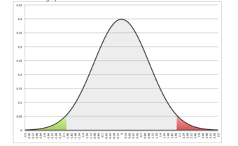
Standard Deviation
This is a normal distribution curve that illustrates standard deviations. The likelihood of being further away from the mean diminishes quickly on both ends.
Expected Value and Standard Error of a Sum
Suppose there are five numbers in a box: 1, 1, 2, 3, and 4. If we were to selected one number from the box, the expected value would be:
![E[X]=1\cdot \frac{1}{5}+1\cdot \frac{1}{5}+2\cdot \frac{1}{5}+3\cdot \frac{1}{5}+4\cdot \frac{1}{5}=2.2](https://open.ocolearnok.org/app/uploads/quicklatex/quicklatex.com-b2cd3101b2d822f38829a33d5e3201ba_l3.png "Rendered by QuickLaTeX.com")
Now, let’s say we draw a number from the box 25 times (with replacement). The new expected value of the sum of the numbers can be calculated by the number of draws multiplied by the expected value of the box: . The standard error of the sum can be calculated by the square root of number of draws multiplied by the standard deviation of the box: . This means that if this experiment were to be repeated many times, we could expect the sum of 25 numbers chosen to be within 5.8 of the expected value of 55, either higher or lower.

7.5.2: Using the Normal Curve
The normal curve is used to find the probability that a value falls within a certain standard deviation away from the mean.
Learning Objective
Calculate the probability that a variable is within a certain range by finding its z-value and using the Normal curve
Key Takeaways
Key Points
- In order to use the normal curve to find probabilities, the observed value must first be standardized using the following formula: .
- To calculate the probability that a variable is within a range, we have to find the area under the curve. Luckily, we have tables to make this process fairly easy.
- When reading the table, we must note that the leftmost column tells you how many sigmas above the the mean the value is to one decimal place (the tenths place), the top row gives the second decimal place (the hundredths), and the intersection of a row and column gives the probability.
- It is important to remember that the table only gives the probabilities to the left of the z-value and that the normal curve is symmetrical.
- In a normal distribution, approximately 68% of values fall within one standard deviation of the mean, approximately 95% of values fall with two standard deviations of the mean, and approximately 99.7% of values fall within three standard of the mean.

Key Terms
- standard deviation
- a measure of how spread out data values are around the mean, defined as the square root of the variance
- z-value
- the standardized value of an observation found by subtracting the mean from the observed value, and then dividing that value by the standard deviation; also called $z$-score
Z-Value
The functional form for a normal distribution is a bit complicated. It can also be difficult to compare two variables if their mean and or standard deviations are different. For example, heights in centimeters and weights in kilograms, even if both variables can be described by a normal distribution. To get around both of these conflicts, we can define a new variable:
This variable gives a measure of how far the variable is from the mean (), then “normalizes” it by dividing by the standard deviation (). This new variable gives us a way of comparing different variables. The -value tells us how many standard deviations, or “how many sigmas”, the variable is from its respective mean.
Areas Under the Curve
To calculate the probability that a variable is within a range, we have to find the area under the curve. Normally, this would mean we’d need to use calculus. However, statisticians have figured out an easier method, using tables, that can typically be found in your textbook or even on your calculator.
| z | 0 | 0.01 | 0.02 | 0.03 | 0.04 | 0.05 | 0.06 | 0.07 | 0.08 | 0.09 |
|---|---|---|---|---|---|---|---|---|---|---|
| 0 | 0.5 | 0.50399 | 0.50798 | 0.51197 | 0.51595 | 0.51994 | 0.52392 | 0.5279 | 0.53188 | 0.53586 |
| 0.1 | 0.53983 | 0.5438 | 0.54776 | 0.55172 | 0.55567 | 0.55962 | 0.5636 | 0.56749 | 0.57142 | 0.57535 |
| 0.2 | 0.57926 | 0.58317 | 0.58706 | 0.59095 | 0.59483 | 0.59871 | 0.60257 | 0.60642 | 0.61026 | 0.61409 |
| 0.3 | 0.61791 | 0.62172 | 0.62552 | 0.6293 | 0.63307 | 0.63683 | 0.64058 | 0.64431 | 0.64803 | 0.65173 |
| 0.4 | 0.65542 | 0.6591 | 0.66276 | 0.6664 | 0.67003 | 0.67364 | 0.67724 | 0.68082 | 0.68439 | 0.68793 |
| 0.5 | 0.69146 | 0.69497 | 0.69847 | 0.70194 | 0.7054 | 0.70884 | 0.71226 | 0.71566 | 0.71904 | 0.7224 |
| 0.6 | 0.72575 | 0.72907 | 0.73237 | 0.73565 | 0.73891 | 0.74215 | 0.74537 | 0.74857 | 0.75175 | 0.7549 |
| 0.7 | 0.75804 | 0.76115 | 0.76424 | 0.7673 | 0.77035 | 0.77337 | 0.77637 | 0.77935 | 0.7823 | 0.78524 |
| 0.8 | 0.78814 | 0.79103 | 0.79389 | 0.79673 | 0.79955 | 0.80234 | 0.80511 | 0.80785 | 0.81057 | 0.81327 |
| 0.9 | 0.81594 | 0.81859 | 0.82121 | 0.82381 | 0.82639 | 0.82894 | 0.83147 | 0.83398 | 0.83646 | 0.83891 |
| 1 | 0.84134 | 0.84375 | 0.84614 | 0.84849 | 0.85083 | 0.85314 | 0.85543 | 0.85769 | 0.85993 | 0.86214 |
| 1.1 | 0.86433 | 0.8665 | 0.86864 | 0.87076 | 0.87286 | 0.87493 | 0.87698 | 0.879 | 0.881 | 0.88298 |
| 1.2 | 0.88493 | 0.88686 | 0.88877 | 0.89065 | 0.89251 | 0.89435 | 0.89617 | 0.89796 | 0.89973 | 0.90147 |
| 1.3 | 0.9032 | 0.9049 | 0.90658 | 0.90824 | 0.90988 | 0.91149 | 0.91308 | 0.91466 | 0.91621 | 0.91774 |
| 1.4 | 0.91924 | 0.92073 | 0.9222 | 0.92364 | 0.92507 | 0.92647 | 0.92785 | 0.92922 | 0.93056 | 0.93189 |
| 1.5 | 0.93319 | 0.93448 | 0.93574 | 0.93699 | 0.93822 | 0.93943 | 0.94062 | 0.94179 | 0.94295 | 0.94408 |
| 1.6 | 0.9452 | 0.9463 | 0.94738 | 0.94845 | 0.9495 | 0.95053 | 0.95154 | 0.95254 | 0.95352 | 0.95449 |
| 1.7 | 0.95543 | 0.95637 | 0.95728 | 0.95818 | 0.95907 | 0.95994 | 0.9608 | 0.96164 | 0.96246 | 0.96327 |
| 1.8 | 0.96407 | 0.96485 | 0.96562 | 0.96638 | 0.96712 | 0.96784 | 0.96856 | 0.96926 | 0.96995 | 0.97062 |
| 1.9 | 0.97128 | 0.97193 | 0.97257 | 0.9732 | 0.97381 | 0.97441 | 0.975 | 0.97558 | 0.97615 | 0.9767 |
| 2 | 0.97725 | 0.97778 | 0.97831 | 0.97882 | 0.97932 | 0.97982 | 0.9803 | 0.98077 | 0.98124 | 0.98169 |
| 2.1 | 0.98214 | 0.98257 | 0.983 | 0.98341 | 0.98382 | 0.98422 | 0.98461 | 0.985 | 0.98537 | 0.98574 |
| 2.2 | 0.9861 | 0.98645 | 0.98679 | 0.98713 | 0.98745 | 0.98778 | 0.98809 | 0.9884 | 0.9887 | 0.98899 |
| 2.3 | 0.98928 | 0.98956 | 0.98983 | 0.9901 | 0.99036 | 0.99061 | 0.99086 | 0.99111 | 0.99134 | 0.99158 |
| 2.4 | 0.9918 | 0.99202 | 0.99224 | 0.99245 | 0.99266 | 0.99286 | 0.99305 | 0.99324 | 0.99343 | 0.99361 |
| 2.5 | 0.99379 | 0.99396 | 0.99413 | 0.9943 | 0.99446 | 0.99461 | 0.99477 | 0.99492 | 0.99506 | 0.9952 |
| 2.6 | 0.99534 | 0.99547 | 0.9956 | 0.99573 | 0.99585 | 0.99598 | 0.99609 | 0.99621 | 0.99632 | 0.99643 |
| 2.7 | 0.99653 | 0.99664 | 0.99674 | 0.99683 | 0.99693 | 0.99702 | 0.99711 | 0.9972 | 0.99728 | 0.99736 |
| 2.8 | 0.99744 | 0.99752 | 0.9976 | 0.99767 | 0.99774 | 0.99781 | 0.99788 | 0.99795 | 0.99801 | 0.99807 |
| 2.9 | 0.99813 | 0.99819 | 0.99825 | 0.99831 | 0.99836 | 0.99841 | 0.99846 | 0.99851 | 0.99856 | 0.99861 |
| 3 | 0.99865 | 0.99869 | 0.99874 | 0.99878 | 0.99882 | 0.99886 | 0.99889 | 0.99893 | 0.99896 | 0.999 |
| 3.1 | 0.99903 | 0.99906 | 0.9991 | 0.99913 | 0.99916 | 0.99918 | 0.99921 | 0.99924 | 0.99926 | 0.99929 |
| 3.2 | 0.99931 | 0.99934 | 0.99936 | 0.99938 | 0.9994 | 0.99942 | 0.99944 | 0.99946 | 0.99948 | 0.9995 |
| 3.3 | 0.99952 | 0.99953 | 0.99955 | 0.99957 | 0.99958 | 0.9996 | 0.99961 | 0.99962 | 0.99964 | 0.99965 |
| 3.4 | 0.99966 | 0.99968 | 0.99969 | 0.9997 | 0.99971 | 0.99972 | 0.99973 | 0.99974 | 0.99975 | 0.99976 |
| 3.5 | 0.99977 | 0.99978 | 0.99978 | 0.99979 | 0.9998 | 0.99981 | 0.99981 | 0.99982 | 0.99983 | 0.99983 |
| 3.6 | 0.99984 | 0.99985 | 0.99985 | 0.99986 | 0.99986 | 0.99987 | 0.99987 | 0.99988 | 0.99988 | 0.99989 |
| 3.7 | 0.99989 | 0.9999 | 0.9999 | 0.9999 | 0.99991 | 0.99991 | 0.99992 | 0.99992 | 0.99992 | 0.99992 |
| 3.8 | 0.99993 | 0.99993 | 0.99993 | 0.99994 | 0.99994 | 0.99994 | 0.99994 | 0.99995 | 0.99995 | 0.99995 |
| 3.9 | 0.99995 | 0.99995 | 0.99996 | 0.99996 | 0.99996 | 0.99996 | 0.99996 | 0.99996 | 0.99997 | 0.99997 |
| 4 | 0.99997 | 0.99997 | 0.99997 | 0.99997 | 0.99997 | 0.99997 | 0.99998 | 0.99998 | 0.99998 | 0.99998 |
Standard Normal Table
This table can be used to find the cumulative probability up to the standardized normal value z. You can use common search engines to find Z-score tables as needed.
These tables can be a bit intimidating, but you simply need to know how to read them. The leftmost column tells you how many sigmas above the the mean to one decimal place (the tenths place).The top row gives the second decimal place (the hundredths).The intersection of a row and column gives the probability.
For example, if we want to know the probability that a variable is no more than 0.51 sigmas above the mean, , we look at the 6th row down (corresponding to 0.5) and the 2nd column (corresponding to 0.01). The intersection of the 6th row and 2nd column is 0.6950, which tells us that there is a 69.50% percent chance that a variable is less than 0.51 sigmas (or standard deviations) above the mean.
A common mistake is to look up a -value in the table and simply report the corresponding entry, regardless of whether the problem asks for the area to the left or to the right of the -value. The table only gives the probabilities to the left of the -value. Since the total area under the curve is 1, all we need to do is subtract the value found in the table from 1. For example, if we wanted to find out the probability that a variable is more than 0.51 sigmas above the mean, , we just need to calculate , or 30.5%.
There is another note of caution to take into consideration when using the table: The table provided only gives values for positive -values, which correspond to values above the mean. What if we wished instead to find out the probability that a value falls below a -value of , or 0.51 standard deviations below the mean? We must remember that the standard normal curve is symmetrical, meaning that , which we calculated above to be 30.5%.
Symmetrical Normal Curve
This images shows the symmetry of the normal curve. In this case, P(z2.01).
We may even wish to find the probability that a variable is between two z-values, such as between 0.50 and 1.50, or P(0.50).
68-95-99.7 Rule
Although we can always use the -score table to find probabilities, the 68-95-99.7 rule helps for quick calculations. In a normal distribution, approximately 68% of values fall within one standard deviation of the mean, approximately 95% of values fall with two standard deviations of the mean, and approximately 99.7% of values fall within three standard deviations of the mean.
68-95-99.7 Rule
Dark blue is less than one standard deviation away from the mean. For the normal distribution, this accounts for about 68% of the set, while two standard deviations from the mean (medium and dark blue) account for about 95%, and three standard deviations (light, medium, and dark blue) account for about 99.7%.
7.4.3: The Correction Factor
The expected value is a weighted average of all possible values in a data set.
Learning Objective
Recognize when the correction factor should be utilized when sampling
Key Takeaways
Key Points
- The expected value refers, intuitively, to the value of a random variable one would “expect” to find if one could repeat the random variable process an infinite number of times and take the average of the values obtained.
- The intuitive explanation of the expected value above is a consequence of the law of large numbers: the expected value, when it exists, is almost surely the limit of the sample mean as the sample size grows to infinity.
- From a rigorous theoretical standpoint, the expected value of a continuous variable is the integral of the random variable with respect to its probability measure.
- A positive value for r indicates a positive association between the variables, and a negative value indicates a negative association.
- Correlation does not necessarily imply causation.
Key Terms
- integral
- the limit of the sums computed in a process in which the domain of a function is divided into small subsets and a possibly nominal value of the function on each subset is multiplied by the measure of that subset, all these products then being summed
- random variable
- a quantity whose value is random and to which a probability distribution is assigned, such as the possible outcome of a roll of a die
- weighted average
- an arithmetic mean of values biased according to agreed weightings
In probability theory, the expected value refers, intuitively, to the value of a random variable one would “expect” to find if one could repeat the random variable process an infinite number of times and take the average of the values obtained. More formally, the expected value is a weighted average of all possible values. In other words, each possible value the random variable can assume is multiplied by its assigned weight, and the resulting products are then added together to find the expected value.
The weights used in computing this average are the probabilities in the case of a discrete random variable (that is, a random variable that can only take on a finite number of values, such as a roll of a pair of dice), or the values of a probability density function in the case of a continuous random variable (that is, a random variable that can assume a theoretically infinite number of values, such as the height of a person).
From a rigorous theoretical standpoint, the expected value of a continuous variable is the integral of the random variable with respect to its probability measure. Since probability can never be negative (although it can be zero), one can intuitively understand this as the area under the curve of the graph of the values of a random variable multiplied by the probability of that value. Thus, for a continuous random variable the expected value is the limit of the weighted sum, i.e. the integral.
Simple Example
Suppose we have a random variable X, which represents the number of girls in a family of three children. Without too much effort, you can compute the following probabilities:
The expected value of X, E[X], is computed as:
![E[X]=\sum_{x=0}^{3}xP[X=x]](https://open.ocolearnok.org/app/uploads/quicklatex/quicklatex.com-658caf3de24bf49c08d94aaeff11385e_l3.png "Rendered by QuickLaTeX.com")
This calculation can be easily generalized to more complicated situations. Suppose that a rich uncle plans to give you $2,000 for each child in your family, with a bonus of $500 for each girl. The formula for the bonus is:
What is your expected bonus?
![E[1000+500X]=\sum_{x=0}^{3}(1000+500x)P[X=x]](https://open.ocolearnok.org/app/uploads/quicklatex/quicklatex.com-d84fc5111f8de6b96a3c779c8b435272_l3.png "Rendered by QuickLaTeX.com")
We could have calculated the same value by taking the expected number of children and plugging it into the equation:
Expected Value and the Law of Large Numbers
The intuitive explanation of the expected value above is a consequence of the law of large numbers: the expected value, when it exists, is almost surely the limit of the sample mean as the sample size grows to infinity. More informally, it can be interpreted as the long-run average of the results of many independent repetitions of an experiment (e.g. a dice roll). The value may not be expected in the ordinary sense—the “expected value” itself may be unlikely or even impossible (such as having 2.5 children), as is also the case with the sample mean.
Uses and Applications
To empirically estimate the expected value of a random variable, one repeatedly measures observations of the variable and computes the arithmetic mean of the results. If the expected value exists, this procedure estimates the true expected value in an unbiased manner and has the property of minimizing the sum of the squares of the residuals (the sum of the squared differences between the observations and the estimate). The law of large numbers demonstrates (under fairly mild conditions) that, as the size of the sample gets larger, the variance of this estimate gets smaller.
This property is often exploited in a wide variety of applications, including general problems of statistical estimation and machine learning, to estimate (probabilistic) quantities of interest via Monte Carlo methods.
The expected value plays important roles in a variety of contexts. In regression analysis, one desires a formula in terms of observed data that will give a “good” estimate of the parameter giving the effect of some explanatory variable upon a dependent variable. The formula will give different estimates using different samples of data, so the estimate it gives is itself a random variable. A formula is typically considered good in this context if it is an unbiased estimator—that is, if the expected value of the estimate (the average value it would give over an arbitrarily large number of separate samples) can be shown to equal the true value of the desired parameter.
In decision theory, and in particular in choice under uncertainty, an agent is described as making an optimal choice in the context of incomplete information. For risk neutral agents, the choice involves using the expected values of uncertain quantities, while for risk averse agents it involves maximizing the expected value of some objective function such as a von Neumann-Morgenstern utility function.
7.4.4: A Closer Look at the Gallup Poll
The Gallup Poll is an opinion poll that uses probability samples to try to accurately represent the attitudes and beliefs of a population.
Learning Objective
Examine the errors that can still arise in the probability samples chosen by Gallup
Key Takeaways
Key Points
- The Gallup Poll has transitioned over the years from polling people in their residences to using phone calls. Today, both landlines and cell phones are called, and are selected randomly using a technique called random digit dialing.
- Opinion polls like Gallup face problems such as nonresponse bias, response bias, undercoverage, and poor wording of questions.
- Contrary to popular belief, sample sizes as small as 1,000 can accurately represent the views of the general population within 4 percentage points, if chosen properly.
- To make sure that the sample is representative of the whole population, each respondent is assigned a weight so that demographic characteristics of the weighted sample match those of the entire population. Gallup weighs for gender, race, age, education, and region.
Key Terms
- probability sample
- a sample in which every unit in the population has a chance (greater than zero) of being selected in the sample, and this probability can be accurately determined
- nonresponse
- the absence of a response
- undercoverage
- Occurs when a survey fails to reach a certain portion of the population.
Overview of the Gallup Poll
The Gallup Poll is the division of Gallup, Inc. that regularly conducts public opinion polls in more than 140 countries around the world. Historically, the Gallup Poll has measured and tracked the public’s attitudes concerning virtually every political, social, and economic issue of the day, including highly sensitive or controversial subjects. It is very well known when it comes to presidential election polls and is often referenced in the mass media as a reliable and objective audience measurement of public opinion. Its results, analyses, and videos are published daily on Gallup.com in the form of data-driven news. The poll has been around since 1935.
How Does Gallup Choose its Samples?
The Gallup Poll is an opinion poll that uses probability sampling. In a probability sample, each individual has an equal opportunity of being selected. This helps generate a sample that can represent the attitudes, opinions, and behaviors of the entire population.
In the United States, from 1935 to the mid-1980s, Gallup typically selected its sample by selecting residences from all geographic locations. Interviewers would go to the selected houses and ask whatever questions were included in that poll, such as who the interviewee was planning to vote for in an upcoming election .

Voter Polling Questionnaire
This questionnaire asks voters about their gender, income, religion, age, and political beliefs.
There were a number of problems associated with this method. First of all, it was expensive and inefficient. Over time, Gallup realized that it needed to come up with a more effective way to collect data rapidly. In addition, there was the problem of non-response. Certain people did not wish to answer the door to a stranger, or simply declined to answer the questions the interviewer asked.
In 1986, Gallup shifted most of its polling to the telephone. This provided a much quicker way to poll many people. In addition, it was less expensive because interviewers no longer had to travel all over the nation to go to someone’s house. They simply had to make phone calls. To make sure that every person had an equal opportunity of being selected, Gallup used a technique called random digit dialing. A computer would randomly generate phone numbers found from telephone exchanges for the sample. This method prevented problems such as under-coverage, which could occur if Gallup had chosen to select numbers from a phone book (since not all numbers are listed). When a house was called, the person over eighteen with the most recent birthday would be the one to respond to the questions.
A major problem with this method arose in the mid-late 2000s, when the use of cell phones spiked. More and more people in the United States were switching to using only their cell phones over landline telephones. Now, Gallup polls people using a mix of landlines and cell phones. Some people claim that the ratio they use is incorrect, which could result in a higher percentage of error.
Sample Size and Error
A lot of people incorrectly assume that in order for a poll to be accurate, the sample size must be huge. In actuality, small sample sizes that are chosen well can accurately represent the entire population, with, of course, a margin of error. Gallup typically uses a sample size of 1,000 people for its polls. This results in a margin of error of about 4%. To make sure that the sample is representative of the whole population, each respondent is assigned a weight so that demographic characteristics of the weighted sample match those of the entire population (based on information from the US Census Bureau). Gallup weighs for gender, race, age, education, and region.
Potential for Inaccuracy
Despite all the work done to make sure a poll is accurate, there is room for error. Gallup still has to deal with the effects of nonresponse bias, because people may not answer their cell phones. Because of this selection bias, the characteristics of those who agree to be interviewed may be markedly different from those who decline. Response bias may also be a problem, which occurs when the answers given by respondents do not reflect their true beliefs. In addition, it is well established that the wording of the questions, the order in which they are asked, and the number and form of alternative answers offered can influence results of polls. Finally, there is still the problem of coverage bias. Although most people in the United States either own a home phone or a cell phone, some people do not (such as the homeless). These people can still vote, but their opinions would not be taken into account in the polls.
Attributions
- Expected Value and Standard Error
-
“Standard deviation diagram.”
http://commons.wikimedia.org/wiki/File:Standard_deviation_diagram.svg.
Wikimedia
CC BY-SA.
- Using the Normal Curve
-
“Using Normal Distributions – IB Math Stuff.”
http://ibmathstuff.wikidot.com/usingnormaldistributions.
Wikidot
CC BY-SA. -
“Standard deviation diagram.”
https://en.wikipedia.org/wiki/File:Standard_deviation_diagram.svg.
Wikipedia
CC BY-SA. -
“Using Normal Distributions – IB Math Stuff.”
http://ibmathstuff.wikidot.com/usingnormaldistributions.
Wikidot
CC BY-SA.
- The Correction Factor
-
“Stats: Expected value and moments (July 29, 2005).”
http://www.pmean.com/05/Moments.asp.
P.Mean Website
CC BY.
- A Closer Look at the Gallup Poll
-
“Nonprobability sampling.”
http://en.wikipedia.org/wiki/Nonprobability_sampling.
Wikipedia
CC BY-SA 3.0.
