This section reviews the fundamental skills for entering formulas into an Excel worksheet. The example used for this chapter is the construction of a personal budget. Most financial advisors recommend that all households construct and maintain a personal budget to achieve and maintain strong financial health. Organizing and maintaining a personal budget is a skill you can practice at any point in your life. Whether you are managing your expenses during college or maintaining the finances of a family of four, a personal budget can be a vital tool when making financial decisions. Excel can make managing your money a fun and rewarding exercise.

Open the Data File

Download Data File: CH2 Data

1. Open the Data file named CH2 Data and use the File/Save As command to save it with the new name CH2 Personal Budget.

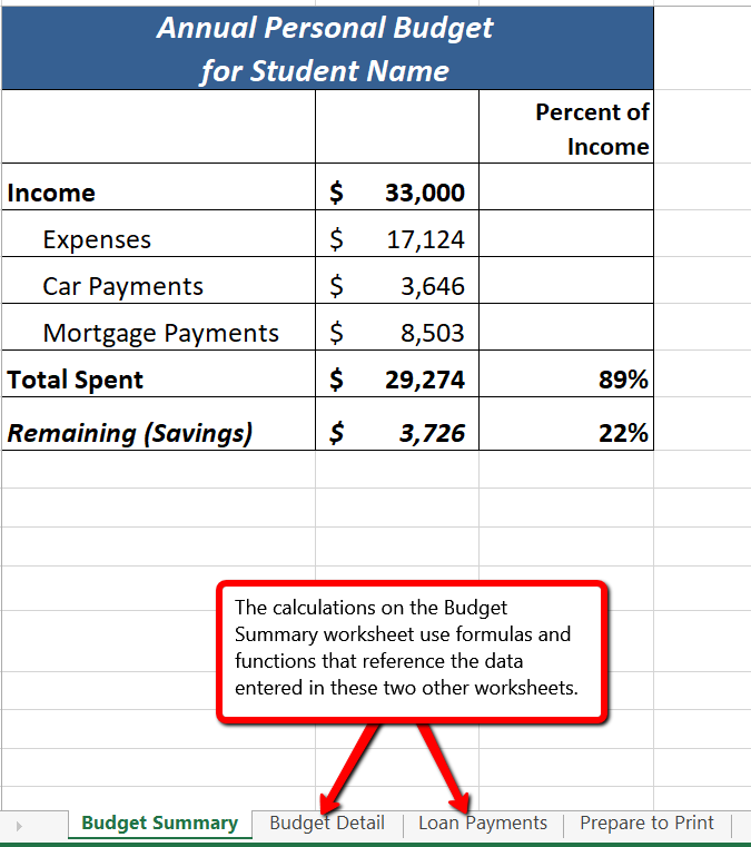
Figure 2.1 shows the completed workbook that will be demonstrated in this chapter. Notice that this workbook contains four worksheets. The first worksheet, Budget Summary, serves as an overview of the data that was entered and calculated in the second and third worksheets, Budget Detail and Loan Payments. The second worksheet, Budget Detail, provides a detailed list of all the expenses and the third worksheet, Loan Payments, provides information regarding car payment and mortgage payment amounts.  The last worksheet, Prepare to Print, has data that is unrelated to the budget worksheets but will be used in Section 2.4 – Preparing to Print.

Creating a Basic Formula

When formulas and cell references are used Excel will automatically recalculate when data is changed

Formulas are used to calculate a variety of mathematical outputs in Excel and can be used to create virtually any custom calculation required for your objective. Furthermore, when constructing a formula in Excel, you use cell addresses that, when added to a formula, become cell references. This means that Excel uses, or references, the number entered into the cell location when performing the calculation. As a result, when the numbers in the cells that are referenced are changed, Excel automatically recalculates the formula and produces a new result. This is what gives Excel the ability to create a variety of what-if scenarios, which will be explained later in the chapter.

To demonstrate the construction of a basic formula, we will begin working on the Budget Detail worksheet, which is shown in Figure 2.2. To complete this worksheet, we will enter some data, and then create several formulas and functions. Table 2.1 provides definitions for each of the spend categories listed in the range A3:A11. When you develop a personal budget, these categories are defined on the basis of how you spend your money. It is likely that every person could have different categories or define the same categories differently. Therefore, it is important to review the definitions in Table 2.1 to understand how we are defining these categories before proceeding.

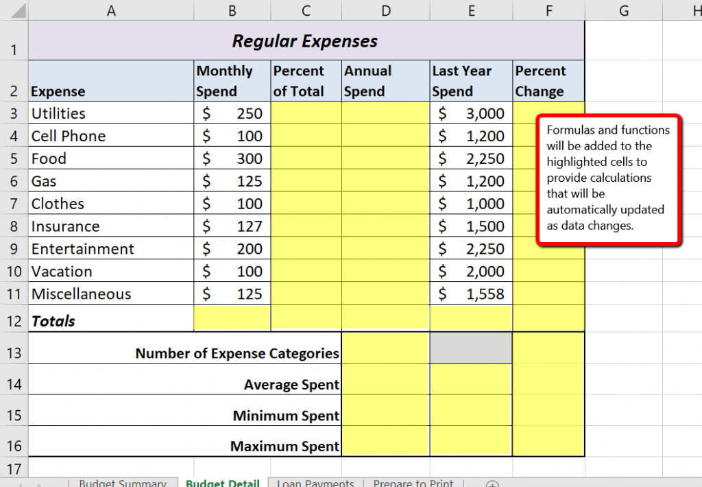
Table 2.1 Spend Category Definitions

Category	Definition
Utilities	Electricity, heat, water, home phone, cable, Internet access
Cell Phone	Cell phone plan and equipment charges
Food	Groceries
Gas	Cost of gas for vehicle
Clothes	Clothes, shoes, and accessories
Insurance	Renter, homeowner, and/or car insurance
Entertainment	Activities like dining out, movie and theater tickets, parties, and so on
Vacation	Vacation expenses
Miscellaneous	Any other spending categories

The amount of money spent each month for each category, as well as the amount of money spent last year, is already entered into the worksheet. We will write formulas that will calculate the annual (yearly) amount spent, the percent of the total spent each category represents, as well as the percent change from last year’s spending to the current year.

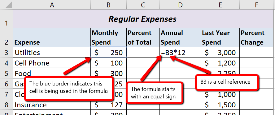
The first formula will calculate the Annual Spend values. The formula will be constructed so that it takes the values in the Monthly Spend column and multiplies them by 12 (the number of months in a year). This will show how much money will be spent per year for each of the categories listed in Column A.  Since the first category is Utilities, we will start by creating the formula to multiply the Monthly Spend amount in B3 by 12. This formula will be created in D3 – the Annual Spend cell for the Utilities category.  This formula will be written as: =B3*12

1. Switch to the Budget Detail worksheet if needed.  Click cell D3.Formulas always start with the equal sign. This signifies to Excel that the contents of the cell should be calculated, not just displayed as basic text or numbers.
2. Type an equal sign =
   When the first character entered into a cell is an equal sign, it signals Excel to perform a calculation.
3. Type B3. This adds B3 to the formula, which is now a cell reference. Excel will use whatever value is entered into cell B3 in the calculation.
4. Type the * . This is the symbol for multiplication in Excel. As shown in Table 2.2 the mathematical operators in Excel are slightly different from those found on a typical calculator.
5. Type the number 12. This multiplies the value in cell B3 by 12. In this formula, a number, or constant, is used instead of a cell reference because it will not change. In other words, there will always be 12 months in a year.
6. Press the ENTER key. This enters the formula into the cell.

Table 2.2 Excel Mathematical Operators (move up)

Symbol	Operation
+	Addition
−	Subtraction
/	Division
*	Multiplication
^	Power/Exponent

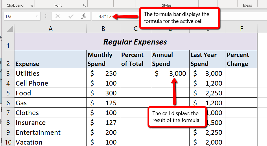
Figure 2.3 shows how the formula appears in cell D3 before you press the ENTER key. Figure 2.4 shows the result of the formula after you press the ENTER key, as well as the formula bar which displays the formula as it was entered in the cell.

The Annual Spend for Utilities is $3,000 because the formula is taking the Monthly Spend in cell B3 and multiplying it by 12. If the value in cell B3 is changed, the formula automatically produces a new result.

Relative References (Copying and Pasting Formulas)

Once a formula is typed into a worksheet, it can be copied and pasted to other cell locations. For example, in cell D3 we have calculated the annual spend for the Utilities category, but this calculation needs to be performed for the rest of the cell locations in Column D. Since we used the B3 cell reference in the formula, Excel automatically adjusts that cell reference when the formula is copied and pasted into the rest of the cell locations in the column. This is called relative referencing and is demonstrated as follows:

1. Click cell D3.
2. Place the mouse pointer over the Auto Fill Handle in the bottom right corner of the cell.
3. When the mouse pointer turns from a white block plus sign to a black plus sign, click and drag down to cell D11. This pastes the formula into the range D4:D11.
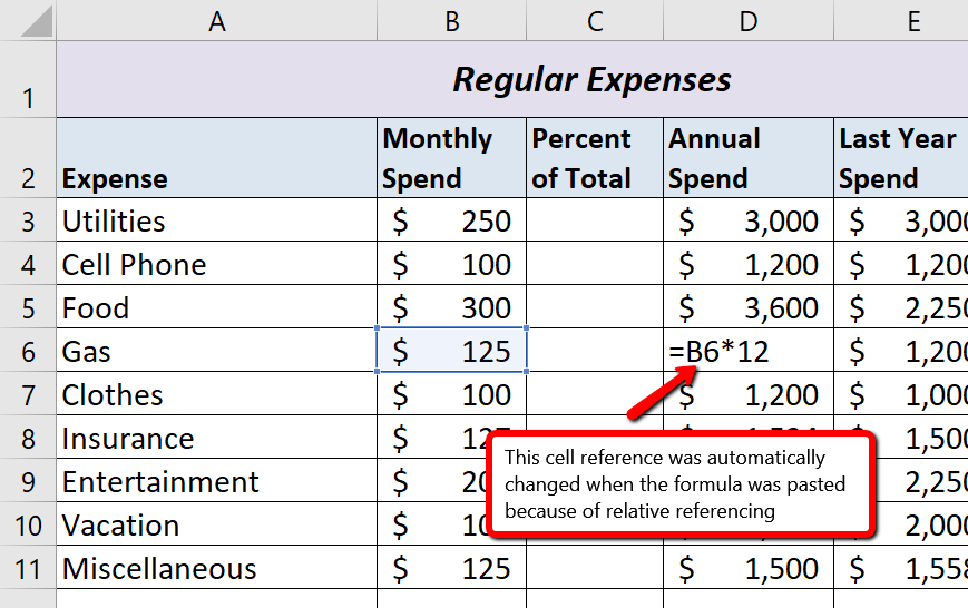
4. Double click cell D6. Notice that the cell reference in the formula is automatically changed to B6.
5. Press the ENTER key.

Figure 2.5 shows the results added to the rest of the cell locations in the Annual Spend column. For each row, the formula takes the value in the Monthly Spend column and multiplies it by 12. You will also see that cell D6 has been double clicked to show the formula. Notice that Excel automatically changed the original cell reference of B3 to B6. This is the result of relative referencing, which means Excel automatically adjusts a cell reference relative to its original location when it is pasted into new cell locations. In this example, the formula was pasted into eight cell locations below the original cell location. As a result, Excel increased the row number of the original cell reference by a value of one for each row it was pasted into.

Creating Complex Formulas (Controlling the Order of Operations)

The next formula to be added to the Personal Budget workbook is the percent change over last year (Column F). This formula determines the difference between this year’s Annual Spend values (Column D) and the values in the Last Year Spend column (Column E) and shows the difference in terms of a percentage. This requires that the order of mathematical operations be controlled to get an accurate result.

Excel uses the standard mathematical order of operations, as defined in Table 2.3.  When writing complex formulas it is important to remember this order of operations. You want to be sure that your formulas will calculate in the order you intend.  To help you remember which operations will be performed first, you can use the acronym PEMDAS.

P – parentheses
E – exponents
MD – multiplication and division
AS – addition and subtraction

Table 2.3 shows the standard order of operations (PEMDAS) for a typical formula. To change the order of operations shown in the table, you can use parentheses to process certain mathematical calculations first.

Table 2.3 Standard Order of Mathematical Operations (PEMDAS)

Symbol	Order
( )	Any calculation inside parentheses will be done first. If there are layers of parentheses used in a formula, Excel computes the innermost parentheses first and the outermost parentheses last.
^	Excel executes any exponential computations next.
* or /	Excel performs any multiplication or division computations next. When there are multiple instances of these computations in a formula, they are executed in order from left to right.
+ or −	Excel performs any addition or subtraction computations last. When there are multiple instances of these computations in a formula, they are executed in order from left to right.

To create the Percent Change formula, we will need to use parentheses to control the order of the calculations. We need the difference of the two values to be found before the division is done, so we will use parentheses around the subtraction portion of the formula to indicate that calculation needs to be done first. This formula is added to the worksheet as follows:

1. Click cell F3 in the Budget Detail worksheet.
2. Type an equal sign =.
3. Type an open parenthesis (.
4. Click cell D3. This will add a cell reference to cell D3 to the formula. When building formulas, you can click cell locations instead of typing them.
5. Type a minus sign −.
6. Click cell E3 to add this cell reference to the formula.
7. Type a closing parenthesis ).
8. Type the slash / symbol for division.
9. Click cell E3. This completes the formula that will calculate the percent change of last year’s actual spent dollars vs. this year’s budgeted spend dollars (see Figure 2.6).
10. Press the ENTER key.
11. Click cell F3 to activate it.
12. Place the mouse pointer over the Auto Fill Handle.
13. When the mouse pointer turns from a white block plus sign to a black plus sign, click and drag down to cell F11. This pastes the formula into the range F4:F11.

Figure 2.6 shows the formula that was added to the Budget Detail worksheet to calculate the percent change in spending. The parentheses were added to this formula to control the order of operations. Any mathematical computations placed in parentheses are executed first before the standard order of mathematical operations (see Table 2.3). In this case, if parentheses were not used, Excel would produce an erroneous result for this worksheet.

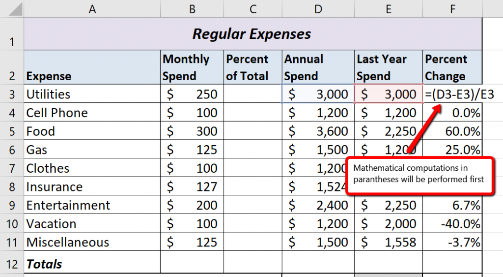
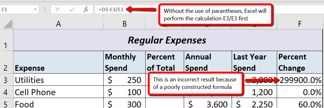
Figure 2.7 shows the result of the percent change formula if the parentheses are removed. The formula produces a result of a 299900% increase. Since there is no change between the LY spend and the budget Annual Spend, the result should be 0%. However, without the parentheses, Excel is following the standard order of operations. This means the value in cell E3 will be divided by E3 first (3,000/3,000), which is 1. Then, the value of 1 will be subtracted from the value in cell D3 (3,000−1), which is 2,999. Since cell F3 is formatted as a percentage, Excel expresses the output as an increase of 299900%.

Auditing Formulas

Excel provides a few tools that you can use to review the formulas entered into a worksheet. For example, instead of showing the outputs for the formulas used in a worksheet, you can have Excel show the formula as it was entered in the cell locations. This is demonstrated as follows:

1. With the Budget Detail worksheet open, click the Formulas tab of the Ribbon.
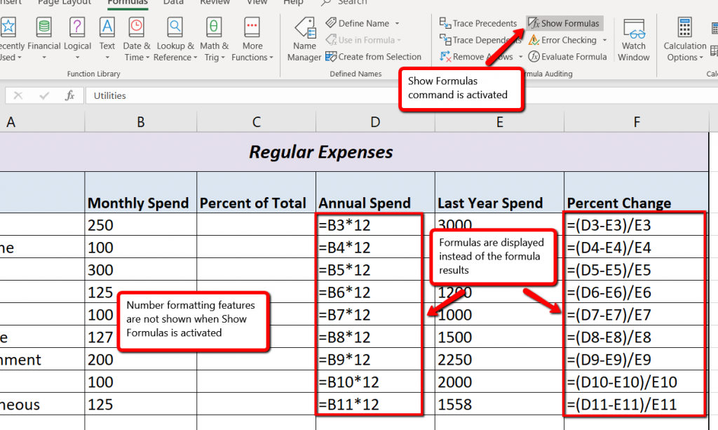
2. Click the Show Formulas button in the Formula Auditing group of commands. This displays the formulas in the worksheet instead of showing the mathematical outputs.
3. Click the Show Formulas button again. The worksheet returns to showing the output of the formulas.

You can also toggle Show Formulas on and off using the keyboard.  Hold down the CTRL key while pressing the ` key.

Figure 2.8 shows the Budget Detail worksheet after activating the Show Formulas command in the Formulas tab of the Ribbon. As shown in the figure, this command allows you to view and check all the formulas in a worksheet without having to click each cell individually. After activating this command, the column widths in your worksheet increase significantly. The column widths were adjusted for the worksheet shown in Figure 2.8 so all columns can be seen. The column widths return to their previous width when the Show Formulas command is deactivated.

Two other tools in the Formula Auditing group of commands are the Trace Precedents and Trace Dependents commands. These commands are used to trace the cell references used in a formula. A precedent cell is a cell whose value is used in other cells. The Trace Precedents command shows an arrow to indicate the cells or ranges (precedents) which affect the active cell’s value. A dependent cell is a cell whose value depends on the values of other cells in the workbook. The Trace Dependents command shows where any given cell is referenced in a formula. The following is a demonstration of these commands:

1. Click cell D3.
2. Click the Trace Dependents button in the Formula Auditing group of commands in the Formulas tab of the Ribbon. A blue arrow appears, pointing to cell F3 (see Figure 2.9). This indicates that cell D3 is referenced in a formula entered in cell F3.
3. Click the Remove Arrows command in the Formula Auditing group of commands in the Formulas tab of the Ribbon. This removes the Trace Dependents arrow.
4. Click cell F3.
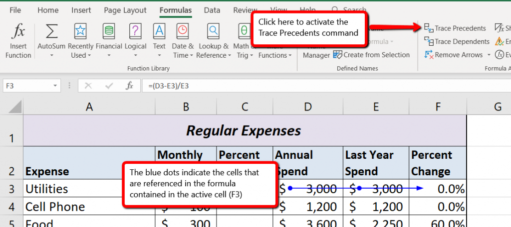
5. Click the Trace Precedents button in the Formula Auditing group of commands in the Formulas tab of the Ribbon. A blue arrow with dots in cells D3 and E3, and pointing to cell F3 appears (see Figure 2.10). This indicates that cells D3 and E3 are references in a formula entered in cell F3.
6. Click the Remove Arrows command in the Formula Auditing group of commands in the Formulas tab of the Ribbon. This removes the Trace Precedents arrow.
7. Save the CH2 Personal Budget file.

Figure 2.9 shows the Trace Dependents arrow on the Budget Detail worksheet. The blue dot represents the activated cell. The arrows indicate where the cell is referenced in formulas.

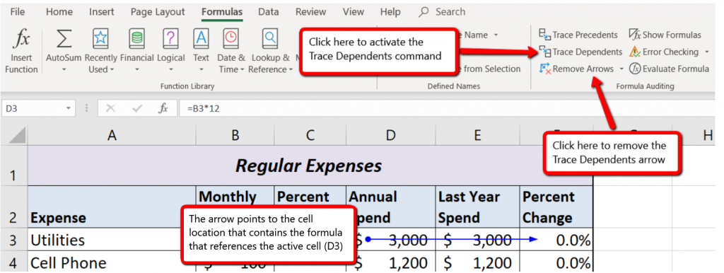
Figure 2.10 shows the Trace Precedents arrow on the Budget Detail worksheet. The blue dots on this arrow indicate the cells that are referenced in the formula contained in the activated cell. The arrow is pointing to the activated cell location that contains the formula.