5.1 Central Tendency
5.1: Central Tendency
5.1.1: Mean: The Average
The term central tendency relates to the way in which quantitative data tend to cluster around some value.
Learning Objectives
Define the average and distinguish between arithmetic, geometric, and harmonic means.
Key Takeaways
Key Points
- An average is a measure of the “middle” or “typical” value of a data set.
- The three most common averages are the Pythagorean means – the arithmetic mean, the geometric mean, and the harmonic mean.
- The arithmetic mean is the sum of a collection of numbers divided by the number of numbers in the collection.
- The geometric mean is a type of mean or average which indicates the central tendency, or typical value, of a set of numbers by using the product of their values. It is defined as the nth root (where n is the count of numbers) of the product of the numbers.
- The harmonic mean H of the positive real numbers X1, X2, … Xn is defined to be the reciprocal of the arithmetic mean of the reciprocals of X1, X2, … Xn. It is typically appropriate for situations when the average of rates is desired.
Key Terms
- average
- any measure of central tendency, especially any mean, the median, or the mode
- arithmetic mean
- the measure of central tendency of a set of values computed by dividing the sum of the values by their number; commonly called the mean or the average
- central tendency
- a term that relates the way in which quantitative data tend to cluster around some value
Example
The arithmetic mean, often simply called the mean, of two numbers, such as 2 and 8, is obtained by finding a value A such that. One may find that  . Switching the order of 2 and 8 to read 8 and 2 does not change the resulting value obtained for A. The mean 5 is not less than the minimum 2 nor greater than the maximum 8. If we increase the number of terms in the list for which we want an average, we get, for example, that the arithmetic mean of 2, 8, and 11 is found by solving for the value of A in the equation
  . One finds that A=7.
The term central tendency relates to the way in which quantitative data tend to cluster around some value. A measure of central tendency is any of a variety of ways of specifying this “central value”. Central tendency is contrasted with statistical dispersion (spread), and together these are the most used properties of distributions. Statistics that measure central tendency can be used in descriptive statistics as a summary statistic for a data set, or as estimators of location parameters of a statistical model.
In the simplest cases, the measure of central tendency is an average of a set of measurements, the word average being variously construed as mean, median, or other measure of location, depending on the context. An average is a measure of the “middle” or “typical” value of a data set. In the most common case, the data set is a list of numbers. The average of a list of numbers is a single number intended to typify the numbers in the list. If all the numbers in the list are the same, then this number should be used. If the numbers are not the same, the average is calculated by combining the numbers from the list in a specific way and computing a single number as being the average of the list.
The term mean has three related meanings:
- The arithmetic mean of a sample,
- The expected value of a random variable, or
- The mean of a probability distribution
The Pythagorean Means
The three most common averages are the Pythagorean means – the arithmetic mean, the geometric mean, and the harmonic mean.

Comparison of Pythagorean Means
Comparison of the arithmetic, geometric and harmonic means of a pair of numbers. The vertical dashed lines are asymptotes for the harmonic means.
The Arithmetic Mean
When we think of means, or averages, we are typically thinking of the arithmetic mean. It is the sum of a collection of numbers divided by the number of numbers in the collection. The collection is often a set of results of an experiment, or a set of results from a survey of a subset of the public. In addition to mathematics and statistics, the arithmetic mean is used frequently in fields such as economics, sociology, and history, and it is used in almost every academic field to some extent. For example, per capita income is the arithmetic average income of a nation’s population.
Suppose we have a data set containing the values a1, …, an. The arithmetic mean is defined via the expression:

If the data set is a statistical population (i.e., consists of every possible observation and not just a subset of them), then the mean of that population is called the population mean. If the data set is a statistical sample (a subset of the population) we call the statistic resulting from this calculation a sample mean. If it is required to use a single number as an estimate for the values of numbers, then the arithmetic mean does this best. This is because it minimizes the sum of squared deviations from the estimate.
The Geometric Mean
The geometric mean is a type of mean or average which indicates the central tendency, or typical value, of a set of numbers by using the product of their values (as opposed to the arithmetic mean which uses their sum). The geometric mean applies only to positive numbers. The geometric mean is defined as the th root (where is the count of numbers) of the product of the numbers.
For instance, the geometric mean of two numbers, say 2 and 8, is just the square root of their product; that is . As another example, the geometric mean of the three numbers 4, 1, and 1/32 is the cube root of their product (1/8), which is 1/2; that is ![\sqrt[3]{4\cdot 1\cdot \frac{1}{32}}=\frac{1}{2}](https://open.ocolearnok.org/app/uploads/quicklatex/quicklatex.com-5605c9445a8cd1228d03bd755c6d3d8d_l3.png "Rendered by QuickLaTeX.com") .
.

A geometric mean is often used when comparing different items – finding a single “figure of merit” for these items – when each item has multiple properties that have different numeric ranges. The use of a geometric mean “normalizes” the ranges being averaged, so that no range dominates the weighting, and a given percentage change in any of the properties has the same effect on the geometric mean.
For example, the geometric mean can give a meaningful “average” to compare two companies which are each rated at 0 to 5 for their environmental sustainability, and are rated at 0 to 100 for their financial viability. If an arithmetic mean was used instead of a geometric mean, the financial viability is given more weight because its numeric range is larger – so a small percentage change in the financial rating (e.g. going from 80 to 90) makes a much larger difference in the arithmetic mean than a large percentage change in environmental sustainability (e.g. going from 2 to 5).
The Harmonic Mean
The harmonic mean is typically appropriate for situations when the average of rates is desired. It may (compared to the arithmetic mean) mitigate the influence of large outliers and increase the influence of small values.
The harmonic mean of the positive real numbers is defined to be the reciprocal of the arithmetic mean of the reciprocals of . For example, the harmonic mean of 1, 2, and 4 is:

The harmonic mean is the preferable method for averaging multiples, such as the price/earning ratio in Finance, in which price is in the numerator. If these ratios are averaged using an arithmetic mean (a common error), high data points are given greater weights than low data points. The harmonic mean, on the other hand, gives equal weight to each data point.
5.1.2: The Average and the Histogram
The shape of a histogram can assist with identifying other descriptive statistics, such as which measure of central tendency is appropriate to use.
Learning Objectives
Demonstrate the effect that the shape of a distribution has on measures of central tendency.
Key Takeaways
Key Points
- Histograms tend to form shapes, which when measured can describe the distribution of data within a dataset.
- A key feature of the normal distribution is that the mode, median and mean are the same and are together in the center of the curve.
- A key feature of the skewed distribution is that the mean and median have different values and do not all lie at the center of the curve.
- Skewed distributions with two or more modes are known as bi-modal or multimodal, respectively.
Key Terms
- normal distribution
- A family of continuous probability distributions such that the probability density function is the normal (or Gaussian) function.
- bell curve
- In mathematics, the bell-shaped curve that is typical of the normal distribution.
- histogram
- A representation of tabulated frequencies, shown as adjacent rectangles, erected over discrete intervals (bins), with an area equal to the frequency of the observations in the interval.
As discussed, a histogram is a bar graph displaying tabulated frequencies. Histograms tend to form shapes, which when measured can describe the distribution of data within a dataset. The shape of the distribution can assist with identifying other descriptive statistics, such as which measure of central tendency is appropriate to use.
The distribution of data item values may be symmetrical or asymmetrical. Two common examples of symmetry and asymmetry are the “normal distribution” and the “skewed distribution. ”
Central Tendency and Normal Distributions
In a symmetrical distribution the two sides of the distribution are a mirror image of each other. A normal distribution is a true symmetric distribution of data item values. When a histogram is constructed on values that are normally distributed, the shape of columns form a symmetrical bell shape. This is why this distribution is also known as a “normal curve” or “bell curve. ” is an example of a normal distribution:
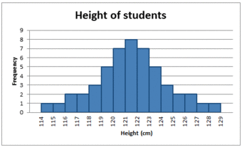
The Normal Distribution
A histogram showing a normal distribution, or bell curve.
If represented as a ‘normal curve’ (or bell curve) the graph would take the following shape (where is the mean and is the standard deviation):
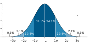
The Bell Curve
The shape of a normally distributed histogram.
A key feature of the normal distribution is that the mode, median and mean are the same and are together in the center of the curve.
Also, there can only be one mode (i.e. there is only one value which is most frequently observed). Moreover, most of the data are clustered around the center, while the more extreme values on either side of the center become less rare as the distance from the center increases (i.e. about 68% of values lie within one standard deviation () away from the mean; about 95% of the values lie within two standard deviations; and about 99.7% are within three standard deviations. This is known as the empirical rule or the 3-sigma rule).
Central Tendency and Skewed Distributions
In an asymmetrical distribution the two sides will not be mirror images of each other. Skewness is the tendency for the values to be more frequent around the high or low ends of the -axis. When a histogram is constructed for skewed data it is possible to identify skewness by looking at the shape of the distribution. For example, a distribution is said to be positively skewed when the tail on the right side of the histogram is longer than the left side. Most of the values tend to cluster toward the left side of the -axis (i.e, the smaller values) with increasingly fewer values at the right side of the -axis (i.e. the larger values).
A distribution is said to be negatively skewed when the tail on the left side of the histogram is longer than the right side. Most of the values tend to cluster toward the right side of the -axis (i.e. the larger values), with increasingly less values on the left side of the -axis (i.e. the smaller values).
A key feature of the skewed distribution is that the mean and median have different values and do not all lie at the center of the curve.
There can also be more than one mode in a skewed distribution. Distributions with two or more modes are known as bi-modal or multimodal, respectively. The distribution shape of the data in is bi-modal because there are two modes (two values that occur more frequently than any other) for the data item (variable).
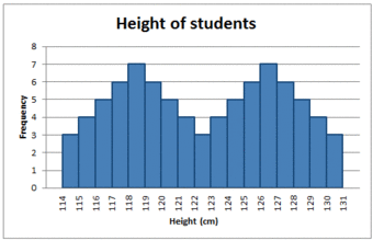
Bi-modal Distribution
Some skewed distributions have two or more modes.
5.1.3: The Root-Mean-Square
The root-mean-square, also known as the quadratic mean, is a statistical measure of the magnitude of a varying quantity, or set of numbers.
Learning Objective
Compute the root-mean-square and express its usefulness.
Key Takeaways
Key Points
- The root-mean-square is especially useful when a data set includes both positive and negative numbers.
- Its name comes from its definition as the square root of the mean of the squares of the values.
- The process of computing the root mean square is to: 1) Square all of the values 2) Compute the average of the squares 3) Take the square root of the average.
- The root-mean-square is always greater than or equal to the average of the unsigned values.
Key Term
- root mean square
- the square root of the arithmetic mean of the squares
The root-mean-square, also known as the quadratic mean, is a statistical measure of the magnitude of a varying quantity, or set of numbers. It can be calculated for a series of discrete values or for a continuously varying function. Its name comes from its definition as the square root of the mean of the squares of the values.
This measure is especially useful when a data set includes both positive and negative numbers. For example, consider the set of numbers . Computing the average of this set of numbers wouldn’t tell us much because the negative numbers cancel out the positive numbers, resulting in an average of zero. This gives us the “middle value” but not a sense of the average magnitude.
One possible method of assigning an average to this set would be to simply erase all of the negative signs. This would lead us to compute an average of 5.6. However, using the RMS method, we would square every number (making them all positive) and take the square root of the average. Explicitly, the process is to:
- Square all of the values
- Compute the average of the squares
- Take the square root of the average
In our example:


The root-mean-square is always greater than or equal to the average of the unsigned values. Physical scientists often use the term “root-mean-square” as a synonym for standard deviation when referring to the square root of the mean squared deviation of a signal from a given baseline or fit. This is useful for electrical engineers in calculating the “AC only” RMS of an electrical signal. Standard deviation being the root-mean-square of a signal’s variation about the mean, rather than about 0, the DC component is removed (i.e. the RMS of the signal is the same as the standard deviation of the signal if the mean signal is zero).

Mathematical Means
This is a geometrical representation of common mathematical means. , are scalars. is the arithmetic mean of scalars and . is the geometric mean, is the harmonic mean, is the quadratic mean (also known as root-mean-square).
5.1.4: Which Average: Mean, Mode, or Median?
Depending on the characteristic distribution of a data set, the mean, median or mode may be the more appropriate metric for understanding.
Learning Objective
Assess various situations and determine whether the mean, median, or mode would be the appropriate measure of central tendency.
Key Takeaways
Key Points
- In symmetrical, unimodal distributions, such as the normal distribution (the distribution whose density function, when graphed, gives the famous “bell curve”), the mean (if defined), median and mode all coincide.
- If elements in a sample data set increase arithmetically, when placed in some order, then the median and arithmetic mean are equal. For example, consider the data sample {1, 2, 3, 4}. The mean is 2.5, as is the median.
- While the arithmetic mean is often used to report central tendencies, it is not a robust statistic, meaning that it is greatly influenced by outliers (values that are very much larger or smaller than most of the values).
- The median is of central importance in robust statistics, as it is the most resistant statistic, having a breakdown point of 50%: so long as no more than half the data is contaminated, the median will not give an arbitrarily large result.
- Unlike mean and median, the concept of mode also makes sense for “nominal data” (i.e., not consisting of numerical values in the case of mean, or even of ordered values in the case of median).
Key Terms
- Mode
- the most frequently occurring value in a distribution
- breakdown point
- the number or proportion of arbitrarily large or small extreme values that must be introduced into a batch or sample to cause the estimator to yield an arbitrarily large result
- median
- the numerical value separating the higher half of a data sample, a population, or a probability distribution, from the lower half
The Mode
The mode is the value that appears most often in a set of data. For example, the mode of the sample is 6. Like the statistical mean and median, the mode is a way of expressing, in a single number, important information about a random variable or a population.
The mode is not necessarily unique, since the same maximum frequency may be attained at different values. Given the list of data the mode is not unique – the dataset may be said to be bimodal, while a set with more than two modes may be described as multimodal. The most extreme case occurs in uniform distributions, where all values occur equally frequently.
For a sample from a continuous distribution, the concept is unusable in its raw form. No two values will be exactly the same, so each value will occur precisely once. In order to estimate the mode, the usual practice is to discretize the data by assigning frequency values to intervals of equal distance, as with making a histogram, effectively replacing the values with the midpoints of the intervals they are assigned to. The mode is then the value where the histogram reaches its peak.
The Median
The median is the numerical value separating the higher half of a data sample, a population, or a probability distribution, from the lower half. The median of a finite list of numbers can be found by arranging all the observations from lowest value to highest value and picking the middle one (e.g., the median of is 5). If there is an even number of observations, then there is no single middle value. In this case, the median is usually defined to be the mean of the two middle values.
The median can be used as a measure of location when a distribution is skewed, when end-values are not known, or when one requires reduced importance to be attached to outliers (e.g., because there may be measurement errors).
Which to Use?
In symmetrical, unimodal distributions, such as the normal distribution (the distribution whose density function, when graphed, gives the famous “bell curve”), the mean (if defined), median and mode all coincide. For samples, if it is known that they are drawn from a symmetric distribution, the sample mean can be used as an estimate of the population mode.
If elements in a sample data set increase arithmetically, when placed in some order, then the median and arithmetic mean are equal. For example, consider the data sample . The mean is 2.5, as is the median. However, when we consider a sample that cannot be arranged so as to increase arithmetically, such as , the median and arithmetic mean can differ significantly. In this case, the arithmetic mean is 6.2 and the median is 4. In general the average value can vary significantly from most values in the sample, and can be larger or smaller than most of them.
While the arithmetic mean is often used to report central tendencies, it is not a robust statistic, meaning that it is greatly influenced by outliers (values that are very much larger or smaller than most of the values). Notably, for skewed distributions, such as the distribution of income for which a few people’s incomes are substantially greater than most people’s, the arithmetic mean may not be consistent with one’s notion of “middle,” and robust statistics such as the median may be a better description of central tendency.
The median is of central importance in robust statistics, as it is the most resistant statistic, having a breakdown point of 50%: so long as no more than half the data is contaminated, the median will not give an arbitrarily large result. Robust statistics are statistics with good performance for data drawn from a wide range of probability distributions, especially for distributions that are not normally distributed. One motivation is to produce statistical methods that are not unduly affected by outliers. Another motivation is to provide methods with good performance when there are small departures from parametric distributions.
Unlike median, the concept of mean makes sense for any random variable assuming values from a vector space. For example, a distribution of points in the plane will typically have a mean and a mode, but the concept of median does not apply.

Unlike mean and median, the concept of mode also makes sense for “nominal data” (i.e., not consisting of numerical values in the case of mean, or even of ordered values in the case of median). For example, taking a sample of Korean family names, one might find that “Kim” occurs more often than any other name. Then “Kim” would be the mode of the sample. In any voting system where a plurality determines victory, a single modal value determines the victor, while a multi-modal outcome would require some tie-breaking procedure to take place.
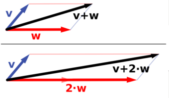
Vector Space
Vector addition and scalar multiplication: a vector (blue) is added to another vector (red, upper illustration). Below, is stretched by a factor of 2, yielding the sum .

Comparison of the Mean, Mode & Median
Comparison of mean, median and mode of two log-normal distributions with different skewness.
5.1.5: Averages of Qualitative and Ranked Data
The central tendency for qualitative data can be described via the median or the mode, but not the mean.
Learning Objective
Categorize levels of measurement and identify the appropriate measures of central tendency.
Key Takeaways
Key Points
- Qualitative data can be defined as either nominal or ordinal.
- The nominal scale differentiates between items or subjects based only on their names and/or categories and other qualitative classifications they belong to.
- The mode is allowed as the measure of central tendency for nominal data.
- The ordinal scale allows for rank order by which data can be sorted, but still does not allow for relative degree of difference between them. The median and the mode are allowed as the measure of central tendency; however, the mean as the measure of central tendency is not allowed.
- The median and the mode are allowed as the measure of central tendency for ordinal data; however, the mean as the measure of central tendency is not allowed.
Key Terms
- quantitative
- of a measurement based on some quantity or number rather than on some quality
- qualitative
- of descriptions or distinctions based on some quality rather than on some quantity
- dichotomous
- dividing or branching into two pieces
Levels of Measurement
In order to address the process for finding averages of qualitative data, we must first introduce the concept of levels of measurement. In statistics, levels of measurement, or scales of measure, are types of data that arise in the theory of scale types developed by the psychologist Stanley Smith Stevens. Stevens proposed his typology in a 1946 Science article entitled “On the Theory of Scales of Measurement. ” In that article, Stevens claimed that all measurement in science was conducted using four different types of scales that he called “nominal”, “ordinal”, “interval” and “ratio”, unifying both qualitative (which are described by his “nominal” type) and quantitative (to a different degree, all the rest of his scales).
Nominal Scale
The nominal scale differentiates between items or subjects based only on their names and/or categories and other qualitative classifications they belong to. Examples include gender, nationality, ethnicity, language, genre, style, biological species, visual pattern, and form.
The mode, i.e. the most common item, is allowed as the measure of central tendency for the nominal type. On the other hand, the median, i.e. the middle-ranked item, makes no sense for the nominal type of data since ranking is not allowed for the nominal type.
Ordinal Scale
The ordinal scale allows for rank order (1st, 2nd, 3rd, et cetera) by which data can be sorted, but still does not allow for relative degree of difference between them. Examples include, on one hand, dichotomous data with dichotomous (or dichotomized) values such as “sick” versus “healthy” when measuring health, “guilty” versus “innocent” when making judgments in courts, or “wrong/false” versus “right/true” when measuring truth value. On the other hand, non-dichotomous data consisting of a spectrum of values is also included, such as “completely agree,” “mostly agree,” “mostly disagree,” and “completely disagree” when measuring opinion .
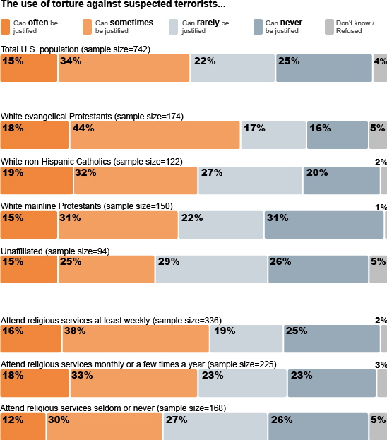
Ordinal Scale Surveys
An opinion survey on religiosity and torture. An opinion survey is an example of a non-dichotomous data set on the ordinal scale for which the central tendency can be described by the median or the mode.
The median, i.e. middle-ranked, item is allowed as the measure of central tendency; however, the mean (or average) as the measure of central tendency is not allowed. The mode is also allowed.
In 1946, Stevens observed that psychological measurement, such as measurement of opinions, usually operates on ordinal scales; thus means and standard deviations have no validity, but they can be used to get ideas for how to improve operationalization of variables used in questionnaires.
Attributions
- Mean: The Average
-
“Measure of central tendency.”
http://en.wikipedia.org/wiki/Measure_of_central_tendency.
Wikipedia
CC BY-SA 3.0. -
“Comparison Pythagorean means.”
http://en.wikipedia.org/wiki/File:Comparison_Pythagorean_means.svg.
Wikipedia
CC BY-SA.
- The Average and the Histogram
-
“Error 404.”
http://www.abs.gov.au/websitedbs/a3121120.nsf/89a5f3d8684682b6ca256de4002c809b/81a53a0a10c05d3bca257949001281b5!OpenDocument.
Austrailian Bureau of Statistics
CC BY. -
“Error 404.”
http://www.abs.gov.au/websitedbs/a3121120.nsf/89a5f3d8684682b6ca256de4002c809b/81a53a0a10c05d3bca257949001281b5!OpenDocument.
Austrailian Bureau of Statistics
CC BY. -
“Error 404.”
http://www.abs.gov.au/websitedbs/a3121120.nsf/89a5f3d8684682b6ca256de4002c809b/81a53a0a10c05d3bca257949001281b5!OpenDocument.
Austrailian Bureau of Statistics
CC BY. -
“Error 404.”
http://www.abs.gov.au/websitedbs/a3121120.nsf/89a5f3d8684682b6ca256de4002c809b/81a53a0a10c05d3bca257949001281b5!OpenDocument.
Austrailian Bureau of Statistics
CC BY.
- The Root-Mean-Square
-
“MathematicalMeans.”
http://commons.wikimedia.org/wiki/File:MathematicalMeans.svg.
Wikimedia
Public domain.
- Which Average: Mean, Mode, or Median?
-
“OpenStax College, Prokaryotic Diversity. October 16, 2013.”
http://cnx.org/content/m44603/latest/Figure_22_01_06.jpg.
OpenStax CNX
CC BY 3.0. -
“Vector addition ans scaling.”
http://commons.wikimedia.org/wiki/File:Vector_addition_ans_scaling.png.
Wikimedia
CC BY-SA. -
“Comparison mean median mode.”
http://commons.wikimedia.org/wiki/File:Comparison_mean_median_mode.svg.
Wikimedia
CC BY-SA.
- Averages of Qualitative and Ranked Data
-
“Religiosity and Torture | Flickr – Photo Sharing!.”
http://www.flickr.com/photos/jurvetson/3492263284/.
Flickr
CC BY.
