15 Factorial ANOVA

Learning Outcomes

In this chapter, you will learn how to:

• Identify when to use a factorial ANOVA
• Conduct an independent measures factorial ANOVA hypothesis test
• Evaluate effect size for an independent measures factorial ANOVA
• Explain main effects and interactions in a two-factor ANOVA
• Evaluate post hoc tests for an independent measures factorial ANOVA
• Identify advantages of an independent measures factorial ANOVA

A single factor ANOVA is the statistical analysis appropriate when we are analyzing the results of a study in which we have one factor and are looking for differences in the response variable among three or more groups or measurement points. We will now review a multi-factor ANOVA, otherwise known as a factorial ANOVA.  We will keep it on the simpler side and use 2-factors (two independent/predictor variables) using a between-groups design.

Logic of a Two-Factor ANOVA

A two factor ANOVA is used when we believe that more than one factor may influence a particular dependent variable. For example, what if we believe that the age of an adolescent will have an impact on number of phone calls made to the opposite sex and we also suspect that the gender of the adolescent will have an impact on the number of phone calls made to the opposite sex.

To test the hypothesis that Age and Gender of adolescent will impact the number of phone calls made to the opposite sex in the past week we would conduct an independent measures factorial ANOVA. In this case, we have a between-groups design for both age and gender.  I have 2 conditions/levels/groups for each factor/variable. I will have to collect data for these for 4 samples of subjects:

Age	Gender
	Young Teen Males	Young Teen Females
	Older Teen Males	Older Teen Females

Table 1. Example of 2×2 ANOVA

A 2×2 ANOVA gives you 4 conditions.  Note: one way to identify the total conditions in a factorial study is to multiply the  number of levels for each factor. Thus, a 2×2 design is 2 times 2 giving us 4 total conditions for the study. We will discuss this more in a moment.

Remember that there are different types of ANOVAs based on design.  In this case, we have a between-groups design.  An individual can only be in 1 condition for gender and 1 condition for age.  So among the 4 total conditions/levels/groups between the 2 factors, an individual is only in 1 of the samples.  For a between-groups design, there are 4 different samples.  Two Factor ANOVA data is commonly organized like the table above which is referred to as a matrix. When the data is organized in a matrix it is very easy to see the factors, as well as the separate levels of the factors.

• Factorial designs like the 2-Factor ANOVA allow a researcher to examine more than one independent variable on the dependent variable
  • Individually for each factor, reporting out a F_test for each. This provides data on the main effect of each independent variable.
  • Collectively where the influence of the factors together is referred to as an interaction. An interaction is the result of the two independent variables combining to produce a result that is different from a result that is produced by either variable alone.

• A 2-Factor ANOVA allows a researcher to assess the main effects (the independent variables) and the interaction yielding three outcomes (3 F_tests), a F_test for factor 1, a F_test for factor 2, and an interaction between factor 1 and 2.

Let’s go back to our example:

• Main Effect of Factor A
  • Is there a significant influence of age of teen (Factor A) on number of phone calls made to the opposite sex (response variable)?  Or, in other words, is there a significant difference between younger teens and older teens in the number of phone calls made to the opposite sex?

• Main Effect of Factor B
  • Is there a significant influence of sex of the teen (Factor B) on number of phone calls made to the opposite sex (response variable)? Or, in other words, is there a significant difference between male and female teens in the number of phone calls made to the opposite sex?

• Interaction of AxB
  • Does the influence of age of teen (Factor A) on the number of phone calls made to the opposite sex (response variable) depend on the sex of the teen (Factor B)?  Or, in other words, is there a significant interaction between age of teen and sex of teen in the number of phone calls made to the opposite sex?

Notice that with two factors we end up with three research questions. Thus, with three research questions, we will have three sets of hypotheses for our hypothesis test.

Conducting a Two Factor ANOVA

Before we begin the process of calculating a 2-Factor ANOVA we need to review several key elements of the study:

• Factors: the independent variables/predictors
• Levels of each factor: how many conditions/groups/treatments a factor has
• Response variable: this is the dependent variable/outcome variable/measurement taken
• Total number of conditions in the experiment: this is identified by multiplying out the number of levels for each factor
• Number of subjects per condition, n: how many participants are in each level/group/treatment
• Total number of participants, N: this will be determined by type of factor for each.

Hypothesis Testing

We use the same steps for two-factor ANOVA that we have used for all other test statistics. However, we will see that there are three separate ANOVA tests yielding three F_tests (fortunately all in a single source table) that are independent and the results are unrelated to the outcome for either of the other two research questions.  As such, we’re going to have three pieces under each of our steps.

Step 1 – State the hypotheses

As mentioned above, since we have three sets of questions, we now have three separate set of hypotheses: one set for each research question:

Main Effect of Factor A

Is there a significant influence of age of teen (Factor A) on number of phone calls made to the opposite sex (response variable)?  Or, in other words, is there a significant difference between younger teens and older teens in the number of phone calls made to the opposite sex?

H₀: μ_{young teens} = μ_{older teens}

H₀: There is not a significant difference between younger and older teens in the number of phone calls made to the opposite sex.

H_A: μ_{young teens} ≠ μ_{older teens}

H_A: There is a significant difference between younger and older teens in the number of phone calls made to the opposite sex.

Main Effect of Factor B

Is there a significant influence of sex of the teen (Factor B) on number of phone calls made to the opposite sex (response variable)? Or, in other words, is there a significant difference between male and female teens in the number of phone calls made to the opposite sex?

H₀: μ_males = μ_females

H₀: There is not a significant difference between male and female teens in the number of phone calls made to the opposite sex.

H_A: μ_males ≠ μ_females

H_A: There is a significant difference between male and female teens in the number of phone calls made to the opposite sex.

Interaction of AxB

Does the influence of age of teen (Factor A) on the number of phone calls made to the opposite sex (response variable) depend on the sex of the teen (Factor B)?  Or, in other words, is there a significant interaction between age of teen and sex of teen in the number of phone calls made to the opposite sex?

H₀: There is not a significant interaction between age and gender of teens in the number of phone calls made to the opposite sex.

H_A: There is a significant interaction between age and gender of teens in the number of phone calls made to the opposite sex.

Step 2 – Find the critical values

There are three research questions, three sets of hypotheses, and eventually three F_test scores so there will be three critical values. The critical boundary of F comes from the F distribution table.

In order to use any F-distribution table, we need to know:

• Alpha (α) – typically chosen between .05 and .01 when using a critical value table.
• degrees of freedom for the denominator, or within treatments = N – (k_A*k_B)
  • In the example data below in Step 3, we see that N = 20, k_A = 2, and k_B = 2.
  • df_{within treatments} = 20 – 2*2 = 20 – 4 = 16
• degrees of freedom for the numerator

This will change depending on which research question we are answering.  The degrees of freedom for the numerator for each research question can be found below.

Main Effect of Factor A

• degrees of freedom for Factor A = df_{A =} (k_A -1) where k_A is number of levels for Factor A
  • Factor A = age which has 2 levels (younger and older)
  • k_A = 2
  • df_A = 2 – 1 = 1
  • F_crit for df 1 and 16 with alpha = .05 is 4.49

Main Effect of Factor B

• degrees of freedom Factor B = df_B = (k_B -1) where k_B is number of levels for Factor B
  • Factor B = gender which has 2 levels (male and female)
  • k_B = 2
  • df_B = 2 – 1 = 1
  • F_crit for df 1 and 16 with alpha = .05 is 4.49

Interaction of AxB

• degrees of freedom Interaction (A x B) = df_AxB = (k_A*k_B – 1) – (k_A-1) – (k_B-1)
  • k_A = 2, k_B = 2
  • df_AxB = (2*2 – 1) – (2 – 1) – (2 – 1) = (4 – 1) – 1 – 1 = 3 – 1 – 1 = 1
  • F_crit for df 1 and 16 with alpha = .05 is 4.49

Note: We would still use the critical value ANOVA table for the critical F-values for each and every hypothesis we’re testing. The critical values may not always be the same for each hypothesis like it was here; it will depend on the number of levels of each factors, the design of the study, and number of participants in each condition!

Step 3 – Calculate the Test Statistics

As in previous chapters, to get to our F_test, we’re going to have to collect our data and create a source table.  This means, we’re going to have to calculate a series of sums of squares and degrees of freedom so that we can then calculate mean square values that can be used to determine our F_test value, or in this case our three F_test values. As you might recall, for a repeated measures one-factor ANOVA, we had to take our within treatments variability and divide it into two parts because we were able to pull our individual differences into our between subjects variability and get a true measure of error. Well, in this example we are back to our independent measures design.  So, we will will be using within treatments variability as our error measure once again. But, now we are looking at three different possible sources of between treatments variability–the main effect of factor A, the main effect of factor B, and the interaction between factor A and factor B. So, what we will see in this example is that instead of divvying up our within treatments variability, we will be divvying up our between treatments or between groups variability.  Let’s remind ourselves what the equations were for sums of squares and degrees of freedom for between treatments (AKA between groups).

As you may recall, the degrees of freedom for between treatments has been the number of levels of the independent variable minus 1.  However, now that we are working with more than 1 independent variable, we have to take this into consideration.  Essentially the between treatments or between groups degrees of freedom is asking how many conditions we are working with minus 1. When we are working with a factorial ANOVA, the number of conditions is calculated by multiplying the number of levels together.

Now that we have the information for our Between Treatments variability, we can divide that into our main effects for factors A and B and our interaction between A and B.

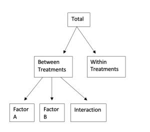
Figure 1. Relationship of variability for two-factor independent measures ANOVA

To calculate our mean square (MS) for our F_tests, we first need to calculate our sums of squares (SS) for our two main effects and our interaction.

Next we can calculate our df values for each of these as well.

Note that our SS and df for our interaction is just our leftover variability from our between treatments.

Next, we need to calculate our sums of squares and degrees of freedom for our within treatments (or error) variability.  This isn’t any different from how we’ve calculated it in past chapters.

Our degrees of freedom are calculated the same as in past chapters as well.  However, the number of treatments is no longer just k, it is now the number of levels in one factor multiplied by the number of levels in the other factor.

Finally, we can check our work by calculating our total sums of squares and total degrees of freedom.

So, now our source table should look like this.

Source	SS	df	MS	F
Between Treatments (bt)	[latex]\sum\frac{T^2}{n}-\frac{G^2}{N}[/latex]	[latex]k_A*k_B-1[/latex]
Factor A (Age)	[latex]\sum\frac{T_A^2}{n_A}-\frac{G^2}{N}[/latex]	[latex]k_A-1[/latex]	[latex]\frac{SS_A}{df_A}[/latex]	[latex]\frac{MS_{A}}{MS_{wt}}[/latex]
Factor B (Gender)	[latex]\sum\frac{T_B^2}{n_B}-\frac{G^2}{N}[/latex]	[latex]k_B-1[/latex]	[latex]\frac{SS_B}{df_A}[/latex]	[latex]\frac{MS_{B}}{MS_{wt}}[/latex]
Interaction (Age x Gender)	[latex]SS_{bt}-{SS_A}-{SS_B}[/latex]	[latex]df_{bt}-{df_A}-{df_B}[/latex]	[latex]\frac{SS_{AxB}}{df_{AxB}}[/latex]	[latex]\frac{MS_{AxB}}{MS_{wt}}[/latex]
Within Treatment (wt)	[latex]\sum{SS_j}[/latex]	[latex]N-(k_A*k_B)[/latex]	[latex]\frac{SS_{wt}}{df_{wt}}[/latex]
Total	[latex]\sum{X^2}-\frac{G^2}{N}[/latex]	[latex]N-1[/latex]

Table 2. ANOVA source table with equations

Now that we have all of our equations, we can look at the data for our example and do our calculations for Step 3.

 

		Gender
		Male	Female
Age	Younger	M = 3	M = 5	Trow1 = 40	N = 20
		T = 15	T = 25		G = 60
		SS = 10	SS = 4		ΣX2 = 256
		n = 5	n = 5
	Older	M = 3	M = 1	Trow2 = 20
		T = 15	T = 5
		SS = 16	SS = 6
		n = 5	n = 5
		Tcol1 = 30	Tcol2 = 30

Table 3. Example data for a 2×2 independent measures ANOVA looking at the age and gender of teens and how many phone calls they made to the opposite sex.

Let’s calculate our SS values for our source table.

[latex]SS_{betweentreatments}=\sum\frac{T^2}{n}-\frac{G^2}{N}[/latex]

[latex]SS_{betweentreatments}=\frac{15^2}{5}+\frac{25^2}{5}+\frac{15^2}{5}+\frac{5^2}{5}-\frac{60^2}{20}=40[/latex]

[latex]SS_A=\sum\frac{T_A^2}{n_A}-\frac{G^2}{N}=\frac{40^2}{10}+\frac{20^2}{10}-\frac{60^2}{20}=20[/latex]

[latex]SS_B=\sum\frac{T_B^2}{n_B}-\frac{G^2}{N}=\frac{30^2}{10}+\frac{30^2}{10}-\frac{60^2}{20}=0[/latex]

[latex]SS_AxB=SS_{betweentreatments}-SS_A-SS_B=40-20-0=20[/latex]

[latex]SS_{withintreatments}=\sum{SS_j}=10+4+16+6=36[/latex]

[latex]SS_{total}=\sum{X^2}-\frac{G^2}{N}=256-\frac{60^2}{20}=76[/latex]

Let’s replace these values in our Source table.

Source	SS	df	MS	F
Between Treatments (bt)	40	[latex]k_A*k_B-1[/latex]
Factor A (Age)	20	[latex]k_A-1[/latex]	[latex]\frac{SS_A}{df_A}[/latex]	[latex]\frac{MS_{A}}{MS_{wt}}[/latex]
Factor B (Gender)	0	[latex]k_B-1[/latex]	[latex]\frac{SS_B}{df_A}[/latex]	[latex]\frac{MS_{B}}{MS_{wt}}[/latex]
Interaction (Age x Gender)	20	[latex]df_{bt}-{df_A}-{df_B}[/latex]	[latex]\frac{SS_{AxB}}{df_{AxB}}[/latex]	[latex]\frac{MS_{AxB}}{MS_{wt}}[/latex]
Within Treatment (wt)	36	[latex]N-(k_A*k_B)[/latex]	[latex]\frac{SS_{wt}}{df_{wt}}[/latex]
Total	76	[latex]N-1[/latex]

Table 4. Source table with SS calculations completed

Now we can complete the formulas for degrees of freedom and fill in the df column in our source table.

[latex]df_{betweentreatments}=k_A*k_B-1=2*2-1=4-1=3[/latex]

 [latex]df_A=k_A-1=2-1=1[/latex]

[latex]df_B=k_B-1=2-1=1[/latex]

[latex]df_{AxB}=df_{bt}-{df_A}-{df_B}=3-1-1=1[/latex]

[latex]df_{withintreatments}=N-(k_A*k_B)=20-(2*2)=20-4=16[/latex]

[latex]df_{total}=N-1=20-1=19[/latex]

Let’s replace these values in our Source table.

Source	SS	df	MS	F
Between Treatments (bt)	40	3
Factor A (Age)	20	1	[latex]\frac{SS_A}{df_A}[/latex]	[latex]\frac{MS_{A}}{MS_{wt}}[/latex]
Factor B (Gender)	0	1	[latex]\frac{SS_B}{df_A}[/latex]	[latex]\frac{MS_{B}}{MS_{wt}}[/latex]
Interaction (Age x Gender)	20	1	[latex]\frac{SS_{AxB}}{df_{AxB}}[/latex]	[latex]\frac{MS_{AxB}}{MS_{wt}}[/latex]
Within Treatment (wt)	36	16	[latex]\frac{SS_{wt}}{df_{wt}}[/latex]
Total	76	19

Table 5. Source table with df calculations completed

Now we can complete the formulas for mean square and fill in the MS column in our source table.

[latex]MS_A=\frac{SS_A}{df_A}=\frac{20}{1}=20[/latex]

[latex]MS_B=\frac{SS_B}{df_B}=\frac{0}{1}=0[/latex]

[latex]MS_AxB=\frac{SS_{AxB}}{df_{AxB}}=\frac{20}{1}=20[/latex]

[latex]MS_{withintreatments}=\frac{SS_{withintreatments}}{df_{withintreatments}}=\frac{36}{16}=2.25[/latex]

Let’s replace these values in our Source table.

Table 7. Source table with F_test calculations completed

Possible outcomes for two-way factorial ANOVA

In a A X B design, there are eight possibilities:

1. A main effect for factor A only
2. A main effect for factor B only
3. Main effects for A and B only
4. A main effect for A, plus an interaction
5. A main effect for B, plus an interaction
6. Main effects for both A and B, plus an interaction
7. An interaction only, no main effects
8. No main effects and no interaction

Figure 2 shows examples of how these findings might look graphing the means of each of the 4 study conditions in a 2×2 design.

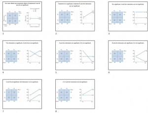
Figure 2. Examples of eight outcomes of a 2×2 ANOVA

Step 4 – Make your decisions

We have three F_test values to work with, so we have three decisions to make. We must compare each of our F_test values to each of our F_crit values determined in Step 2.

Main Effect of A

For the main effect of A or our factor of Age, our F_crit = 4.49 with degrees of freedom numerator of 1 and degrees of freedom denominator of 16.  Our F_test was F(1, 16) = 8.89.  And, 8.89 is greater than 4.49, which means that 8.89 is in our critical region. So, our decision for the main effect of A or the main effect of age in this example is to reject the null hypothesis.

Main Effect of B

For the main effect of B or our factor of Gender, our F_crit = 4.49 with degrees of freedom numerator of 1 and degrees of freedom denominator of 16.  Our F_test was F(1, 16) = 0.  And, 0 is less than 4.49, which means that 0 is NOT in our critical region. So, our decision for the main effect of B or the main effect of gender in this example is to fail to reject the null hypothesis.

Interaction of AxB

For the interaction of AxB or the interaction between our factors of Age and Gender, our F_crit = 4.49 with degrees of freedom numerator of 1 and degrees of freedom denominator of 16.  Our F_test was F(1, 16) = 8.89.  And, 8.89 is greater than 4.49, which means that 8.89 is in our critical region. So, our decision for the interaction of AxB or the interaction of age by gender in this example is to reject the null hypothesis.

Since we found significance for at least one of these F_test values, we need to calculate effect sizes for the ones that were significant.

Calculate effect size

Effect size is calculated for each F_test that is statistically significant. Just like in previous chapters it is reported eta-square. Remember that eta-square is the percentage of total variance explained variance by the factor.  Again, just as you have a F for factor A, a F for factor B, and an F for the interaction, you would have eta-squares for each. But, just like with repeated measures ANOVA, we will be partitioning out the total variability between our main effects and interaction, so we will actually be calculating partial η².

So, for our example, we need to calculate partial eta-squared for two out of our three F_test values.

Main Effect of Age

[latex]partial-η^2=\frac{20}{20+36}=\frac{20}{56}=.36[/latex]

Interaction of Age by Gender

[latex]partial-η^2=\frac{20}{20+36}=\frac{20}{56}=.36[/latex]

Note that we don’t calculate a partial eta-squared for the main effect of gender because we didn’t find a significant effect for that factor. We use the same size cutoffs as before for this measure.

partial-𝜂2	Size
0.01-0.09	Small
0.09-0.25	Medium
0.25+	Large

Table 8. Cut scores for partial eta-squared sizes.

So, what does all of this mean?  How do we interpret three different research questions and sets of hypotheses in one hypothesis test?

Remember, interaction means that the effect of one factor depends on the level of a second factor – so then there is no consistent main effect. If you get a significant interaction, emphasize that finding over any significant main effects. In other words, if there is an interaction effect, then the main effect cannot be discussed without a qualifier. Thus, if we find a significant interaction, we always focus on interpreting the interaction. We report the findings (significant or not) of the main effects, but we interpret the interaction.

So, we are able to explain 36% of the variance in the number of phone calls made to the opposite sex is based on the interaction between gender and age of the teen. Let’s write up what we have so far.

We can conclude that there are significant differences in the number of phone calls made to the opposite sex based on age of the teen, F(1, 16) = 8.89, p < .05, partial-η² = 0.36, but there is not a significant difference due to gender of teen, F(1, 16) = 0.00, p > .05. There is a large significant interaction between age and gender of teen in the number of phone calls made to the opposite sex, F(1, 16) = 8.89, p < .05, partial-η² = 0.36.

Because there were 2×2=4 groups of teens in this study, we need to conduct a post hoc test to determine where these significant differences in this interaction truly lie. And, we will also see that we can graph our data to get an even better picture of the significant interaction we found.

Graphing the Results of Factorial Experiments

The results of factorial experiments with two independent variables can be graphed by representing one independent variable on the x-axis and representing the other by using different kinds of bars or lines. The y-axis is always reserved for the dependent variable.

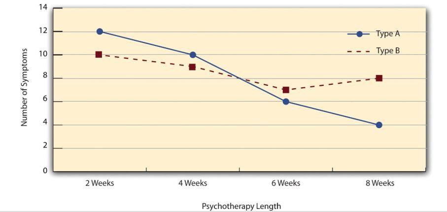
Figure 3. A 4 (Psychotherapy Length) x 2 (Type) ANOVA.

The figure above is a line graph that shows results for a hypothetical 4 x 2 factorial experiment Psychotherapy length, is represented along the x-axis and has four levels (e.g., 2 weeks, 4 weeks, 6 weeks and 8 weeks) and the other variable (psychotherapy type) is represented by differently formatted lines. When we graph our results, we’re able to see the interaction and interpret the results of our study better. For example, in this graph we can see that the Type A Psychotherapy saw a greater reduction over time, while the Type B saw a slower reduction with a slight increase in symptoms at the end of 8 weeks.

Let’s see what a graph for our hypothesis test looks like. We graph the means for the different conditions, with the levels of one factor on our x-axis, and the levels of the other factor in our legend separating our two lines.

	Gender
	Males	Females
Younger teens	M = 3	M = 5
Older teens	M = 3	M = 1

Table 9. Means for hypothesis test example data

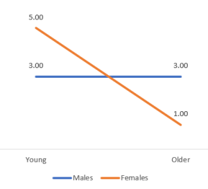
Figure 4. Age x Gender of Teens Factorial ANOVA Graph

As we can see in the graph, for males the average number of phone calls did not change no matter how old they were. However, for the females as they got older the average number of phone calls reduced. Now when we conduct our post hoc test we should see significant differences that reflect this. Note that we don’t need to do a post hoc test for our Main Effects 1) because we had a significant interaction, but 2) because both factors only had 2 levels.

Post hoc tests for Independent Measures Factorial ANOVA

The final step in any hypothesis test with more than three groups or measurement points being compared that are found to be significantly different is a post hoc test. While you can test for simple main effects, we are also familiar with running a Tukey’s post hoc test to test for mean differences between the conditions to see which conditions are significantly different from each other. Let’s continue that tradition here.

In our example we are comparing four conditions, so our table is much bigger than we’ve had in the past.  Below are the differences between the group means, and because we know that each condition has 5 people, we can figure out HSD using the first equation above. Because we had an alpha level of .05, df_{within treatments} = 16, and k = 4, we can find that we can use a q = 4.046 from a Studentized Range critical value table.

[latex]HSD=q\sqrt\frac{MS_{withintreatments}}{n}=4.046\sqrt\frac{2.25}{5}[/latex]

[latex]HSD=4.046\sqrt{0.45}=4.046*0.671=2.71[/latex]

Now, we compare each paired comparison’s mean difference to this value of 2.71.  If it is larger than this value (if the numerical difference is bigger than this number, signs do not matter), then we can say that the two groups are significantly different from each other.

Comparison	Mean Difference	Tukey’s HSD = 2.71
Young Females vs. Old Females	5 – 1 = 4	4 > 2.71  **
Young Females vs. Old Males	5 – 3 = 2	2 < 2.71
Young Females vs. Young Males	5 – 3 = 2	2 < 2.71
Old Females vs. Young Males	1 – 3 = -2 –> 2	2 < 2.71
Old Females vs. Old Males	1 – 3 = -2 –> 2	2 < 2.71
Young Males vs. Old Males	3 – 3 = 0	0 < 2.71

As we can see, only one of the paired comparisons have mean differences greater than Tukey’s HSD, so we can conclude that only the young females are significantly different from the older female teens.  No other pairs were significantly different from any other group.

Assumptions

Depending on the type of factorial design you use, that is which types of factors (independent measures and/or repeated measures) the same assumptions must be met as in previous ANOVAs: normality, independence of observations, homogeneity of variance, and/or sphericity.