9 Introduction to Hypothesis Testing
Learning outcomes
In this chapter, you will learn how to:
- Identify the components of a hypothesis test.
- State the hypotheses and identify appropriate critical areas.
- Describe the proper interpretations of a p-value as well as common misinterpretations.
- Distinguish between the two types of error in hypothesis testing.
- Conduct a hypothesis test using a z-score statistics.
- Explain the purpose of measuring effect size.
- Compute to Cohen's d.
- Identify the assumption underlying a test statistic.
In the first unit we discussed the three major goals of statistics:
- Describe
- Decide
- Predict
The last two goals are related to the idea of hypothesis testing and inferential statistics, while the first is clearly tied to descriptive statistics. The remaining chapters will cover many different kinds of hypothesis tests connected to different inferential statistics. There is a lot of new language we will learn about when conducting a hypothesis test. Some of the components of a hypothesis test are the topics we are already familiar with: probability and distribution of sample means.
Hypothesis testing is an inferential procedure that uses data from a sample to draw a general conclusion about a population. When interpreting a research question and statistical results, a natural question arises as to whether the finding could have occurred by chance. In this chapter, we will introduce the ideas behind the use of statistics to make decisions – in particular, decisions about whether a particular hypothesis is supported by the data.
Logic and Purpose of Hypothesis Testing
Let's consider an example. The case study Physicians' Reactions sought to determine whether physicians spend less time with obese patients. Physicians were sampled randomly and each was shown a chart of a patient complaining of a migraine headache. They were then asked to estimate how long they would spend with the patient. The charts were identical except that for half the charts, the patient was obese and for the other half, the patient was of average weight. The chart a particular physician viewed was determined randomly. Thirty-three physicians viewed charts of average-weight patients and 38 physicians viewed charts of obese patients.
The mean time physicians reported that they would spend with obese patients was 24.7 minutes as compared to a mean of 31.4 minutes for normal-weight patients. How might this difference between means have occurred? One possibility is that physicians were influenced by the weight of the patients. On the other hand, perhaps by chance, the physicians who viewed charts of the obese patients tend to see patients for less time than the other physicians. Random assignment of charts does not ensure that the groups will be equal in all respects other than the chart they viewed. In fact, it is certain the groups differed in many ways by chance. The two groups could not have exactly the same mean age. Perhaps a physician's age affects how long physicians see patients. There are many differences between the groups that could affect how long they view patients. With this in mind, is it plausible that these chance differences are responsible for the difference in times?
To assess the plausibility of the hypothesis that the difference in mean times is due to chance, we compute the probability of getting a difference as large or larger than the observed difference (31.4 - 24.7 = 6.7 minutes) if the difference were, in fact, due solely to chance. Using methods presented in later chapters, this probability can be computed to be 0.0057. Since this is such a low probability, we have confidence that the difference in times is due to the patient's weight and is not due to chance.
In hypothesis testing, like the example described above, we see these four components:
- We create two hypotheses: the null and the alternative.
- We collect and analyze data.
- We determine how likely or unlikely the original hypothesis is to occur based on probability.
- We determine if we have enough evidence to support or reject the null hypothesis and draw conclusions.
Now let's bring in some specific terminology.
Null hypothesis
In general, the null hypothesis, written H0 (“H-naught”), is the idea that nothing is going on: there is no effect of our treatment, no relation between our variables, and no difference in our sample mean from what we expected about the population mean. The null hypothesis indicates that an apparent effect is due to chance. This is always our baseline starting assumption, and it is what we (typically) seek to reject.
In the Physicians' Reactions example, the null hypothesis is that in the population of physicians, the mean time expected to be spent with obese patients is equal to the mean time expected to be spent with average-weight patients. This null hypothesis can be written as:
H0: μobese = μaverage
Alternative hypothesis
If the null hypothesis is rejected, then we will need some other explanation, which we call the alternative hypothesis, HA. The alternative hypothesis is simply the opposite of the null hypothesis. Thus, our alternative hypothesis is the mathematical way of stating our research question. In general, the alternative hypothesis is that there is a significant effect of the treatment, significant relationship between variables, or significant difference between groups. The alternative hypothesis essentially shows evidence the findings are not due to chance. It is also called the research hypothesis as this is the most common outcome a researcher is looking for: evidence of change, differences, or relationships. There are three options for setting up the alternative hypothesis, depending on where we expect the difference to lie. The alternative hypothesis always involves some kind of inequality (≠ "not equal", > "greater than", or < "less than").
-
If we expect a specific direction of change/differences/relationships, which we call a directional hypothesis, then our alternative hypothesis takes the form based on the research question itself. The directional hypothesis (2 directions) makes up 2 of the 3 alternative hypothesis options.
-
The other alternative is to state there are differences/changes, or a relationship but not predict the direction. We use a non-directional hypothesis (typically see ≠ for mathematical notation).
In the Physicians' Reactions example, the directional alternative hypothesis must go in one or the other direction (i.e., more or less time with the obese patients). Based on our research question, the directional alternative hypothesis is that in the population of physicians, the mean time expected to be spent with obese patients is less than the mean time expected to be spent with average-weight patients. This alternative null hypothesis can be written as:
HA: μobese < μaverage
In the Physicians' Reactions example, the non-directional alternative hypothesis simply states that there is difference in time spent with obese patients compared to average-weight patients. This alternative null hypothesis can be written as:
HA: μobese ≠ μaverage
Critical values, p-values, and significance level
A low probability value casts doubt on the null hypothesis. How low must the probability value be in order to conclude that the null hypothesis is very unlikely? Although there is clearly no right or wrong answer to this question, it is conventional to say the null hypothesis is false if the probability value is less than 0.05. More conservative researchers conclude the null hypothesis is false only if the probability value is less than 0.01. When a researcher concludes that the null hypothesis is false, the researcher is said to have "rejected the null hypothesis." The probability value below which the null hypothesis is rejected is called the α level or simply α (“alpha”). It is also called the significance level. If α is not explicitly specified, we often assume that α = 0.05.
The significance level (AKA alpha level) is a threshold we set before collecting data in order to determine whether or not we should reject the null hypothesis. We set this value beforehand to avoid biasing ourselves by viewing our results and then determining what criteria we should use. If our data produce values that meet or exceed this threshold, then we have sufficient evidence to reject the null hypothesis; if not, we fail to reject the null (we never “accept” the null).
There are two criteria we use to assess whether our data meet the thresholds established by our chosen significance level, and they both have to do with our discussions of probability and distributions. Recall that probability refers to the likelihood of an event, given some situation or set of conditions. In hypothesis testing, that situation is the assumption that the null hypothesis value is the correct value, or that there is no effect. The value laid out in H0 is our condition under which we interpret our results. To reject this assumption, and thereby reject the null hypothesis, we need results that would be very unlikely if the null was true.
Now recall that values of z which fall in the tails of the standard normal distribution represent unlikely values. That is, the proportion of the area under the curve as or more extreme than z is very small as we get into the tails of the distribution. Our significance level corresponds to the area under the tail that is exactly equal to α: if we use our normal criterion of α = .05, then 5% of the area under the curve becomes what we call the critical region of the distribution. This is illustrated in Figure 1.
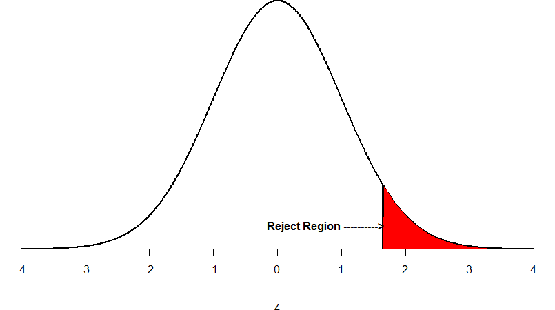
Figure 1. The critical region for a one-tailed test
The shaded rejection region takes up 5% of the area under the curve. Any result which falls in that region is sufficient evidence to reject the null hypothesis.
The critical region is bounded by a specific z-value, as is any area under the curve. In hypothesis testing, the value corresponding to a specific rejection region is called the critical value, zcrit (“z-crit”). Finding the critical value works exactly the same as finding the z-score corresponding to any area under the curve. If we go to the normal table, we will find that the z-score corresponding to 5% of the area under the curve is equal to 1.645 (z = 1.64 corresponds to 0.0505 and z = 1.65 corresponds to 0.0495, so .05 is exactly in between them) if we go to the right and -1.645 if we go to the left. The direction must be determined by your alternative hypothesis, and drawing then shading the distribution is helpful for keeping directionality straight.
Suppose, however, that we want to do a non-directional test. We need to put the critical region in both tails, but we don’t want to increase the overall size of the rejection region (for reasons we will see later). To do this, we simply split it in half so that an equal proportion of the area under the curve falls in each tail’s rejection region. For α = .05, this means 2.5% of the area is in each tail, which, based on the z-table, corresponds to critical values of zcrit = ±1.96. This is shown in Figure 2.
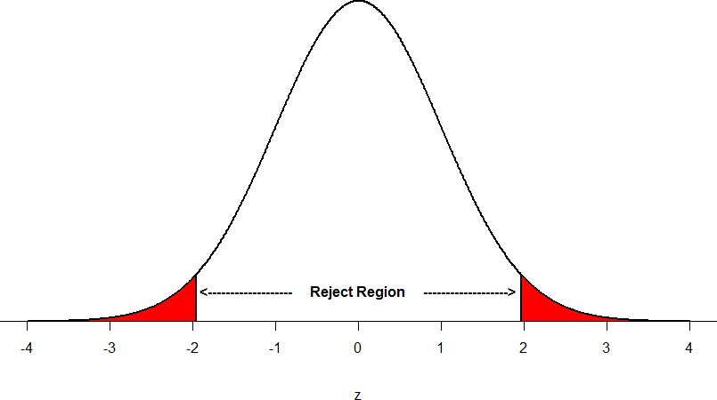
Figure 2. Two-tailed critical region
Thus, any z-score falling outside ±1.96 (greater than 1.96 in absolute value) falls in the critical region.
Choosing one-tail vs two-tail test |
| How do you choose whether to use a one-tailed versus a two-tailed test? The two-tailed test is always going to be more conservative, so it’s always a good bet to use that one, unless you had a very strong prior reason for using a one-tailed test. In that case, you should have written down the hypothesis before you ever looked at the data. It is important that you always come up with your hypotheses before you ever see the actual data. You should never make a decision about how to perform a hypothesis test once you have looked at the data, as this can introduce serious bias into the results. |
To formally test our hypothesis, we must be able to compare an obtained z-statistic to our critical z-value. We call this calculated or obtained z-score our z-test (ztest). If |ztest| > |zcrit| then our sample falls in the critical region (to see why, draw a line for z = 2.5 on Figure 1 or Figure 2), and so we reject H0. If |ztest| < |zcrit|, then we fail to reject H0.
Calculating our Test Statistic
[latex]z_{test}=\frac{M-μ_M}{𝜎_M}[/latex]
Remember, according to the definition of the distribution of sample means:
[latex]μ_M=μ[/latex]
[latex]𝜎_M=\frac{𝜎}{\sqrt{n}}[/latex]
The test statistic is very useful when we are doing our calculations by hand. However, when we use computer software, it will report to us a p-value, which is simply the proportion of the area under the curve in the tails beyond our obtained test statistic. We can directly compare this p-value to α to test our null hypothesis: if p < α, we reject H0, but if p > α, we fail to reject H0.
Thus, as ztest gets farther from zero, the corresponding area under the curve beyond ztest gets smaller. Thus, the proportion, or p-value, will be smaller than the area for α, and if the area is smaller, the probability gets smaller. Specifically, the probability of obtaining that result, or a more extreme result, under the condition that the null hypothesis is true gets smaller.
When the null hypothesis is rejected, the effect is said to be statistically significant. For example, in the Physicians Reactions case study, the probability value is 0.0057 (p = .0057, which means that p < .05). Therefore, the effect of obesity on physicians' reactions is statistically significant and the null hypothesis that obesity makes no difference is rejected. It is very important to keep in mind that statistical significance means only that the null hypothesis no effect is rejected; it does not mean that the effect is important, which is what “significant” usually means. When an effect is significant, you can have confidence the effect is not exactly zero. Finding that an effect is statistically significant does not tell you about how large or important the effect is.
Do not confuse statistical significance with practical significance.
A small effect can be highly significant if the sample size is large enough.
Why does the word “significant” in the phrase “statistically significant” mean something so different from other uses of the word? Interestingly, this is because the meaning of “significant” in everyday language has changed. It turns out that when the procedures for hypothesis testing were developed, something was “significant” if it signified something. Thus, finding that an effect is statistically significant signifies that the effect is most likely real and not due to chance. Over the years, the meaning of “significant” changed, leading to the potential misinterpretation.
Steps of the Hypothesis Testing Process
The process of testing hypotheses follows a simple four-step procedure. This process will be what we use for the remainder of the textbook, and although the hypotheses and statistics we use will change, this process will not.
Step 1: State the Hypotheses
Your hypotheses are the first things you need to lay out. Otherwise, there is nothing to test! You have to state the null hypothesis (which is what we test) and the alternative hypothesis (which is what we expect). These should be stated mathematically as they were presented above AND in words, explaining what each one means in terms of the research question.
Step 2: Find the Critical Values
Next, we formally lay out the criteria we will use to test our hypotheses. There are two pieces of information that inform our critical values: α, which determines how much of the area under the curve composes our critical region, and the directionality of the test, which determines where the region will be.
Step 3: Compute the Test Statistic
Once we have our hypotheses and the standards we use to test them, we can collect data and calculate our test statistic, in this case z. This step is where the vast majority of differences in future chapters will arise: different tests used for different data are calculated in different ways, but the way we use and interpret them remains the same.
Step 4: Make and Interpret the Decision
Finally, once we have our obtained test statistic, we can compare it to our critical value and decide whether we should reject or fail to reject the null hypothesis.
When we do this, we must interpret the decision in relation to our research question, stating what we concluded, what we based our conclusion on, and the specific statistics we obtained (in APA format usually).
Example: Movie Popcorn
Let’s see hypothesis testing in action by working through an example. Say that a movie theater owner likes to keep a very close eye on how much popcorn goes into each bag sold, so he knows that the average bag has 8 cups of popcorn and that this varies a little bit, about half a cup. That is, the known population mean is μ = 8.00 and the known population standard deviation is σ = 0.50. The owner wants to make sure that the newest employee is filling bags correctly, so over the course of a week he randomly assesses 25 bags filled by the employee to test for a difference (n = 25). He doesn’t want bags overfilled or under filled. This scenario has all of the information we need to begin our hypothesis testing procedure.
Step 1: State the Hypotheses
First, we need to decide if we are looking for directional or non-directional hypotheses. In the scenario outlined above, the manager is interested in examining whether bags were "overfilled or underfilled" which implies he wants to look at both directions, which means he's not looking for a particular direction. Thus, this hypothesis test is non-directional. We will need both a null and an alternative hypothesis written both mathematically and in words. We’ll always start with the null hypothesis:
H0: There is no difference in the weight of popcorn bags from this employee
H0: μ = 8.00
Notice that we phrase the hypothesis in terms of the population parameter μ, which in this case would be the true average weight of bags filled by the new employee. Our assumption of no difference, the null hypothesis, is that this mean is exactly the same as the known population mean value we want it to match, 8.00.
Now let’s do the alternative:
HA: There is a difference in the weight of popcorn bags from this employee
HA: μ ≠ 8.00
In this case, we don’t know if the bags will be too full or not full enough, so we do a two-tailed (non-directional) alternative hypothesis that there is a difference.
Step 2: Find the Critical Values
Our critical values are based on two things: the directionality of the test and the significance level or alpha. (Remember, traditional alpha levels are .05, .01, and .001.) We decided in Step 1 that a two-tailed test is the appropriate directionality. We were given no information about the level of significance, so we will assume that α = 0.05. As stated earlier in the chapter, the critical values for a two-tailed z-test at α = 0.05 are zcrit = ±1.96. We can now draw out our distribution (see Figure 3) so we can visualize the critical region and make sure it makes sense.
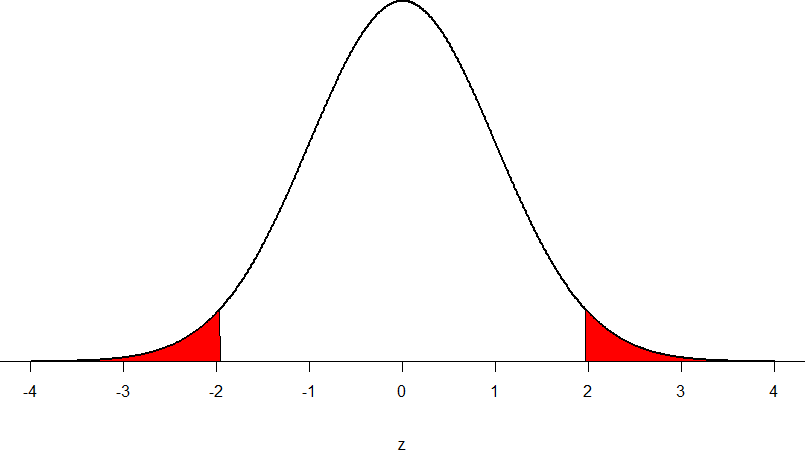
Figure 3. Critical region for zcrit = ±1.96 shaded in red
Step 3: Calculate the Test Statistic
Now we come to our formal calculations. Let’s say that the manager collects data and finds that the average weight of this employee’s n = 25 popcorn bags is M = 7.75 cups.
We can now plug this value, along with the values presented in the original problem, into our equation for ztest:
[latex]z_{test}=\frac{M-μ}{σ_M}=\frac{M-μ}{\frac{σ}{\sqrt{n}}}[/latex]
[latex]z_{test}=\frac{7.75-8.00}{\frac{0.5}{\sqrt{25}}}[/latex]
[latex]z_{test}=\frac{-0.25}{\frac{0.5}{5}}=\frac{-0.25}{0.10}=-2.50[/latex]
Our test statistic is ztest = -2.50, which we can now draw onto our critical region (see Figure 4).
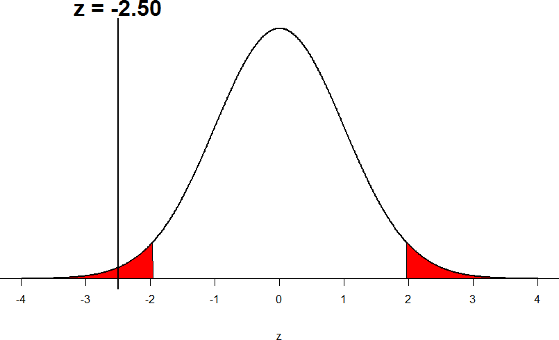
Figure 4. Test statistic location compared to the critical region
Step 4: Make and Interpret the Decision
Looking at Figure 4, we can see that our obtained z-test falls in the critical region. We can also directly compare it to our critical value: in terms of absolute value, |-2.50| > |-1.96|, so we reject the null hypothesis. We can now write our conclusion:
Reject H0. Based on the sample of 25 bags, we can conclude that the average popcorn bag from this employee is significantly smaller (M = 7.75 cups) than the average weight of popcorn bags at this movie theater, z = - 2.50, p < 0.05.
When we write our conclusion, we write out the words to communicate what it actually means, but we also include the average sample size we calculated (the descriptive statistics like we've seen before) and the test statistic and p-value (the inferential statistics we are now learning to calculate). We don’t know the exact p-value, but we do know that because it was in the critical region and we rejected the null, it must be less than α.
Effect Size
When we reject the null hypothesis, we are stating that the difference we found was statistically significant, but we have mentioned several times that this tells us nothing about practical significance. To get an idea of the actual size of the difference, relationship, or effect that we found, we can compute a new inferential statistic called an effect size. Effect sizes give us an idea of how large, important, or meaningful a statistically significant effect is. For the difference between two means as in a z-statistic hypothesis test like we calculated here, our effect size is Cohen’s d.
Calculating Cohen's d
[latex]d=\bigg |\frac{M-μ}{𝜎}\bigg |[/latex]
Note: Because we don't care about the direction of Cohen's d, we take the absolute value of the calculation.
This is very similar to our formula for z, but we no longer take into account the sample size (since overly large samples can make it too easy to reject the null). Cohen’s d is interpreted in units of standard deviations, just like a z-score. For our hypothesis test example above, we rejected the null hypothesis, so we should next ask ourselves, how big of an effect or difference was there? Let's find out.
[latex]d=\bigg |\frac{7.75-8.00}{0.50}\bigg |=\bigg |\frac{-0.25}{0.50}\bigg |=|-0.50|=0.50[/latex]
Cohen’s d is interpreted as small, moderate, or large. Specifically, d = 0.20 is small, d = 0.50 is moderate, and d = 0.80 is large. Obviously values can fall in between these guidelines, so we should use our best judgment and the context of the problem to make our final interpretation of size. Our effect size happened to be exactly equal to one of these, so we say that there was a moderate effect.
| d | Interpretation |
|---|---|
| 0.0 - 0.2 | negligible |
| 0.2 - 0.5 | small |
| 0.5 - 0.8 | medium |
| 0.8 + | large |
Table 1. Interpretation of Cohen's d
Now we can update the report of our findings from above.
Reject H0. Based on the sample of 25 bags, we can conclude that the average popcorn bag from this employee is significantly smaller (M = 7.75 cups) than the average weight of popcorn bags at this movie theater, z = - 2.50, p < 0.05, d = 0.50.
Effect sizes are incredibly useful and provide important information and clarification that overcomes some of the weakness of hypothesis testing. Whenever you find a significant result, you should always calculate and report an effect size.
Other Considerations in Hypothesis Testing
There are several other considerations we need to keep in mind when performing hypothesis testing.
Errors in Hypothesis Testing
In the Physicians' Reactions case study, the probability value associated with the significance test is 0.0057. Therefore, the null hypothesis was rejected, and it was concluded that physicians intend to spend less time with obese patients. Despite the low probability value, it is possible that the null hypothesis is actually true and that the large difference between sample means occurred by chance. If this is the case, then the conclusion that physicians intend to spend less time with obese patients is in error. This type of error is called a Type I error. More generally, a Type I error occurs when a hypothesis test results in the rejection of a true null hypothesis.
The Type I error rate is affected by the α level: the lower the α level the lower the Type I error rate. It might seem that α is the probability of a Type I error. However, this is not correct. Instead, α is the probability of a Type I error given that the null hypothesis is true. If the null hypothesis is false, then it is impossible to make a Type I error.
The second type of error that can be made in significance testing is failing to reject a false null hypothesis. This kind of error is called a Type II error. Unlike a Type I error, a Type II error is not really an error. When a statistical test is not significant, it means that the data do not provide strong evidence that the null hypothesis is false. Lack of significance does not support the conclusion that the null hypothesis is true. Therefore, a researcher should not make the mistake of incorrectly concluding that the null hypothesis is true when a statistical test was not significant. Instead, the researcher should consider the test inconclusive. Contrast this with a Type I error in which the researcher erroneously concludes that the null hypothesis is false when, in fact, it is true.
A Type II error can only occur if the null hypothesis is false. If the null hypothesis is false, then the probability of a Type II error is called β (beta). The probability of correctly rejecting a false null hypothesis equals 1- β and is called power. Power is simply our ability to correctly detect an effect that exists. It is influenced by the size of the effect (larger effects are easier to detect), the significance level we set (making it easier to reject the null makes it easier to detect an effect, but increases the likelihood of a Type I Error), and the sample size used (larger samples make it easier to reject the null).
Summing up, when you perform a hypothesis test, there are four possible outcomes depending on the actual truth (or falseness) of the null hypothesis H0 and the decision to reject or not. The outcomes are summarized in the following table:
| H0 IS ACTUALLY | ||
| ACTION | True | False |
| Do not reject H0 | Correct Outcome | Type II error |
| Reject H0 | Type I Error | Correct Outcome |
Table 2. The four possible outcomes in hypothesis testing.
- The decision is not to reject H0 when H0 is true (correct decision).
- The decision is to reject H0 when H0 is true (incorrect decision known as a Type I error).
- The decision is not to reject H0 when, in fact, H0 is false (incorrect decision known as a Type II error).
- The decision is to reject H0 when H0 is false (correct decision).
Misconceptions in Hypothesis Testing
Misconceptions about hypothesis testing are common. This section lists three important ones.
Misconception #1: The probability value is the probability that the null hypothesis is false.
False. The probability value is the probability of a result as extreme or more extreme given that the null hypothesis is true. It is the probability of the data given the null hypothesis. It is not the probability that the null hypothesis is false.
Misconception#2: A low probability value indicates a large effect.
False. A low probability value indicates that the sample outcome (or one more extreme) would be very unlikely if the null hypothesis were true. A low probability value can occur with small effect sizes, particularly if the sample size is large.
Misconception #3: A non-significant outcome means that the null hypothesis is probably true.
False. A non-significant outcome means that the data do not conclusively demonstrate that the null hypothesis is false.
Misconception #4: A significant outcome means that you have proven your alternative hypothesis to be true.
False. A significant outcome means that you have found evidence to support your alternative hypothesis. We NEVER prove anything to be true! A future study may find something different.
Test Statistic Assumptions
There is one last consideration we will revisit with each test statistic throughout the book--assumptions. There are four main assumptions. These assumptions are often taken for granted in using prescribed data in a statistics course. In the real world, these assumptions would need to be examined and tested using statistical software.
Random Sampling
A sample is random when each person (or animal) in your population has an equal chance of being included in the sample; therefore selection of any individual happens by chance, rather than by choice. This reduces the chance that differences in characteristics or conditions may bias results. Remember that random samples are more likely to be representative of the population so researchers can be more confident interpreting the results. Note: there is no test that statistical software can perform which assures random sampling has occurred, but following good sampling techniques helps to ensure your samples are random.
Independence
Statistical independence is a critical assumption for many statistical tests. It is assumed that observations are independent of each other often but often this assumption. Is not met. Independence means the value of one observation does not influence or affect the value of other observations. Independent data items are not connected with one another in any way (unless you account for it in your study). Even the smallest dependence in your data can turn into heavily biased results (which may be undetectable) if you violate this assumption. Note: there is no test statistical software can perform that assures independence of the data because this should be addressed during the research planning phase. Using a non-parametric test is often recommended if a researcher is concerned this assumption has been violated.
Normality
Normality assumes that the continuous variables (dependent variable) used in the analysis are normally distributed. Normal distributions are symmetric around the center (the mean) and form a bell-shaped distribution. Normality is violated when sample data are skewed. With large enough sample sizes (n > 30) the violation of the normality assumption should not cause major problems (remember the central limit theorem) but there is a feature in most statistical software that can alert researchers to an assumption violation.
Equality of Variances AKA Homoscedasticity
Variance refers to the spread of scores from the mean. Many statistical tests assume that although different samples can come from populations with different means, they have the same variance. Equality of variances (i.e., homogeneity of variance) is violated when variances across different groups or samples are significantly different. Note: there is a feature in most statistical software to test for this.
a statistical inference procedure for determining whether a given proposition about a population parameter should be rejected on the basis of observed sample data.
a statement that a study will find no meaningful differences between the groups or conditions under investigation.
a statement that a study will find meaningful differences or relationships between the variables under investigation.
a scientific prediction stating (a) that an effect will occur and (b) whether that effect will specifically increase or specifically decrease, depending on changes to the independent variable.
a scientific prediction stating that an effect, difference or relationship will occur but does not predict if it will be an increase or decrease.
the portion of a probability distribution containing the values for a test statistic that would result in rejection of a null hypothesis in favor of its corresponding alternative hypothesis.
a value used to make decisions about whether a test result is statistically meaningful.
the numerical result of a statistical test, which is used to determine statistical significane and evaluate the viability of a hypothesis.
the degree to which a research outcome cannot reasonably be attributed to the operation of chance or random factors. It is determined during significance testing and given by a critical p value, which is the probability of obtaining the observed data if the null hypothesis (i.e., of no significant relationship between variables) were true.
A measure of the magnitude or meaningfulness of a difference, relationship, or effect in a study. Often, effect sizes are interpreted as indicating the practical or meaningful significance of a research finding.
When a researcher rejects the null hypothesis when it should not be rejected. Researchers make this error when they believe they have found an effect, difference, or relationship that does not actually exist. The probability of committing a Type I error is called the significance level or alpha (α) level.
When researchers fail to reject the null hypothesis when it is should be rejected. Researchers make this error if they conclude that a particular effect, difference, or relationship does not exist when in fact it does. The probability of committing a Type II error is called the beta (β) level of a test. Conversely, the probability of not committing a Type II error (i.e., of detecting a genuinely significant difference, effect, or relationship) is called the power of the test, where power = 1 – β.
A statistical measure of how effective a statistical procedure is at identifying real differences in a study. It is the probability that use of the procedure will lead to the null hypothesis being rejected.
the condition in which the occurrence of one event makes it neither more nor less probable that another event will occur.
the condition in which a data set presents a normal distribution of values.
the statistical assumption of equal variance, meaning that the average squared distance of a score from the mean is the same across all groups sampled in a study.
