8 Sampling Distributions

Learning outcomes:

In this chapter, you will learn how to:

• Explain a sampling distribution of sample means.
• Define the Central Limit Theorem.
• Describe the law of large numbers.

We have come to the final chapter in this unit. We will now take the logic, ideas, and techniques we have developed and put them together to see how we can take a sample of data and use it to make inferences about what’s truly happening in the broader population. This is the final piece of the puzzle that we need to understand in order to have the groundwork necessary for formal hypothesis testing. Though some of the concepts in this chapter seem familiar, they are really extensions of what we have already learned in previous chapters.

People, Samples, and Populations

In previous chapters we discussed how to find the location of individual scores within a sample’s distribution via z-scores. We also learned that we can extend that to decide how likely it is to observe scores higher or lower than an individual score using probability. All of these principles carry forward from scores within samples to samples within populations. Just like an individual score can differ from its sample mean, an individual sample mean can differ from the true population mean.

We encountered this principle in earlier chapters: sampling error. Sampling error is an incredibly important principle. We know ahead of time that if we collect data and compute a sample statistic, the observed value describing that sample will likely be slightly different from the population parameter; this is natural and expected. However, if our sample statistic is extremely different from what we expected based on the population parameter, there may be something worth examining. One common example where we look for sampling error is the sample mean compared to the population mean.

The Sampling Distribution of Sample Means

To see how we use sampling error, we will learn about a new, theoretical distribution known as the sampling distribution of sample means (often just stated as the “sampling distribution”). In the same way that we can gather a lot of individual scores and put them together to form a distribution, if we were to take many samples, all of the same size, and calculate the mean of each of those, we could put those means together to form a distribution. This new distribution is, intuitively, known as the distribution of sample means. It is one example of what we call a sampling distribution; it can be formed from a set of any statistic, such as a mean, a test statistic, or a correlation coefficient (more on those in later units). For our purposes, understanding the distribution of sample means will be enough to see how all other sampling distributions work to enable and inform our inferential analyses, so these two terms will be used interchangeably from here on out. Let’s take a deeper look at some of its characteristics.

Characteristics of the Sampling Distribution

• The shape of our sampling distribution is normal.
• The center is the mean or average of the means which is equal to the true population mean, μ. It is often called the expected value of M, denoted μ_M.
• The spread is called the standard error, 𝜎_M. The formula for standard error is seen in the box below.

Notice that the sample size is in this equation. As stated above, the sampling distribution refers to samples of a specific size. That is, all sample means must be calculated from samples of the same size n, such n = 10, n = 30, or n = 100. This sample size refers to how many people or observations are in each individual sample, not how many samples are used to form the sampling distribution. This is because the sampling distribution is a theoretical distribution, not one we will ever actually calculate or observe. And, just as a sampling distribution is theoretical, sampling error is the theoretical or conceptual idea that a sample will never quite represent a population perfectly, while standard error is the statistical or calculated measure of that expected difference between our population and our sample means. Figure 1 displays the principles stated here in graphical form.

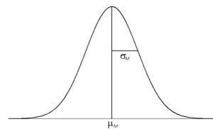
Figure 1. The sampling distribution of sample means

Two Important Axioms

We just learned that the sampling distribution is theoretical: we never actually see it. If that is true, then how can we know it works? How can we use something that we don’t see? The answer lies in two very important mathematical facts: the Central Limit Theorem and the law of large numbers. We will not go into the math behind how these statements were derived, but knowing what they are and what they mean is important to understanding why inferential statistics work and how we can draw conclusions about a population based on information gained from a single sample.

Central Limit Theorem

The central limit theorem states:

For samples of a single size (n), drawn from a population with a given mean (μ) and standard deviation (σ), the sampling distribution of sample means will have a mean (𝜇_M) equal to the population mean and standard deviation (σ_M) equal to the standard error. This distribution will approach normality as n increases.

The last sentence of the central limit theorem states that the sampling distribution will be normal as the sample size of the samples used to create it increases. What this means is that bigger samples will create a more normal distribution, so we are better able to use the techniques we developed for normal distributions and probabilities. So how large is large enough? In general, a sampling distribution will be normal if either of two characteristics is true:

1. The population from which the samples are drawn is normally distributed, or
2. The sample size is equal to or greater than 30.

This second criteria is very important because it enables us to use methods developed for normal distributions even if the true population distribution is skewed.

Law of Large Numbers

The law of large numbers simply states that as our sample size increases, the probability that our sample mean is an accurate representation of the true population mean also increases. It is the formal mathematical way to state that larger samples are more representative of our population.

The law of large numbers is related to the central limit theorem, specifically the formulas for variance and standard error. Remember that the sample size appears in the denominators of those formulas. A larger denominator in any fraction means that the overall value of the fraction gets smaller (i.e., 1/2 = 0.50, 1/3 = 0.33, 1/4 = 0.25, and so on). Thus, larger sample sizes will create smaller standard errors. We already know that standard error is the spread of the sampling distribution and that a smaller spread creates a narrower distribution. Therefore, larger sample sizes create narrower sampling distributions, which increases the probability that a sample mean will be close to the center and decreases the probability that it will be in the tails. This is illustrated in Figures 2 and 3.

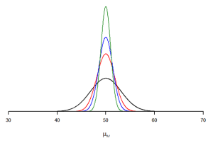
Figure 2. Sampling distributions from the same population with μ = 50 and σ = 10 but different sample sizes (n = 10, black; n = 30, red; n = 50, blue; n = 100, green)

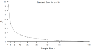
Figure 3. Relation between sample size and standard error for a constant σ = 10

Finding Probability for Sample means

We saw in Chapter 6 that we can use z-scores to split up a normal distribution and calculate the proportion of the area under the curve in one of the new regions, giving us the probability of randomly selecting a z-score under that area of the distribution. We can follow the exact same process for sample means, by converting sample means into z-scores and calculating probabilities. The only difference is that instead of dividing a raw score by the standard deviation, we divide a sample mean by the standard error.

Let’s say we are drawing samples from a population with a mean of 50 and standard deviation of 10 (the same values used in Figure 2). What is the probability that we get a random sample with n = 10 with a mean greater than or equal to 55?

That is, for n = 10, what is the probability that M ≥ 55? First, we need to convert this sample mean score into a z-score:

[latex]z=\frac{55 - 50}{\frac{10}{\sqrt{10}}}=\frac{5}{3.16}=1.58[/latex]

Now we need to shade the area under the normal curve corresponding to scores greater than z = 1.58 as in Figure 4. This area is referred to as the tail.

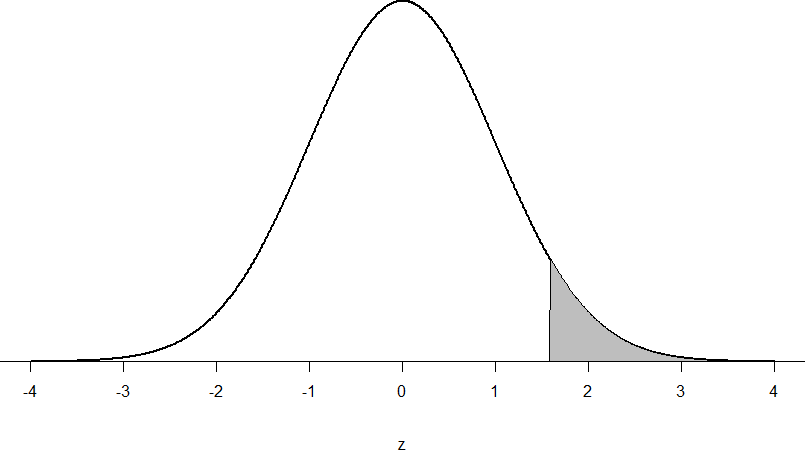
Figure 4: Area under the curve greater than z = 1.58

Now we go to our z-table and find that the area in the tail is = 0.0571. So, the probability of randomly drawing a sample of 10 people from a population with a mean of 50 and standard deviation of 10 whose sample mean is 55 or more is p = .0571, or 5.71%. Notice that we are talking about means that are 55 or more. That is because, strictly speaking, it’s impossible to calculate the probability of a score taking on exactly 1 value since the “shaded region” would just be a line with no area to calculate.

Now let’s do the same thing, but assume that instead of only having a sample of 10 people we took a sample of 50 people. First, we find z:

[latex]z=\frac{55 - 50}{\frac{10}{\sqrt{50}}}=\frac{5}{1.41}=3.55[/latex]

Then we shade the appropriate region of the normal distribution:

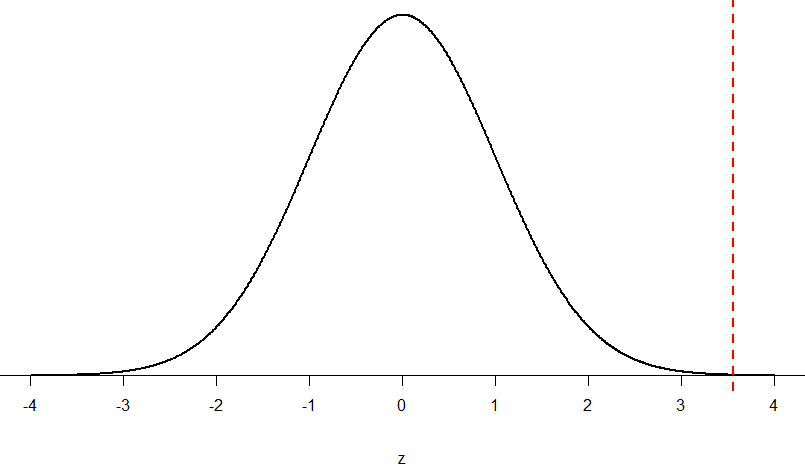
Figure 5: Area under the curve greater than z = 3.55

Notice that no region of Figure 5 appears to be shaded. That is because the area under the curve that far out into the tail is so small that it can’t even be seen (the red line has been added to show exactly where the region starts). Thus, we already know that the probability must be smaller for n = 50 than n = 10 because the size of the area (the proportion) is much smaller.

We run into a similar issue when we try to find z = 3.55 on our Standard Normal Distribution Table. The table goes up to 3.50 and then skips to 3.60, then 3.70, 3.80, 3.90, etc., because everything beyond that is almost 0 and changes so little that it’s not worth printing values. The closest we can get is subtracting the largest value, 0.9990, from 1 to get 0.001. We know that, technically, the actual probability is smaller than this (since 3.55 is farther into the tail than 3.09), so we say that the probability is p < 0.001, or less than 0.1%.  And this is likely why the APA handbook tells us not to report anything more specific than “p < .001” for these probabilities.

This example shows what an impact sample size can have. From the same population, looking for exactly the same thing, changing only the sample size took us from roughly a 5% chance to a less than 0.1% chance (or less than 1 in 1,000). As the sample size n increased, the standard error decreased, which in turn caused the value of z to increase, which finally caused the p-value (a term for probability we will use a lot in later units) to decrease. You can think of this relation like gears: turning the first gear (sample size) clockwise causes the next gear (standard error) to turn counterclockwise, which causes the third gear (z) to turn clockwise, which finally causes the last gear (probability) to turn counterclockwise. All of these pieces fit together, and the relations will always be the same:

n↑ 𝜎_M↓ z↑ p↓

Recap

We’ve seen how we can use the standard error to determine probability based on our normal curve. We can think of the standard error as how much we would naturally expect our statistic – be it a mean or some other statistic – to vary from our parameter. In our formula for z based on a sample mean, the numerator (M − 𝜇_M) is what we call an observed effect. That is, it is what we observe in our sample mean versus what we expected based on the population from which that sample mean was calculated.

Because the sample mean will naturally move around due to sampling error, our observed effect will also change naturally. In the context of our formula for z, then, our standard error is how much we would naturally expect the observed effect to change. Changing by a little is completely normal, but changing by a lot might indicate something is going on. This is the basis of inferential statistics and the logic behind hypothesis testing, which we will introduce in the next chapter.

Before we move on to the next chapter, you might want to practice a bit with z-scores, probability, and the normal distribution table. Here’s another example similar to the one before. For the same population as discussed previously of mean 50 and standard deviation 10, what proportion of sample means fall below 47 if they are of sample size n = 10? What about sample size n = 50?

1. First, you’ll want to calculate z-scores.
2. It can be helpful to sketch a normal distribution and mark the z-score and shade the area under the curve that you are looking for.
3. Compare those z-scores to a normal distribution table.