7 Probability

Learning Outcomes:

Probability can seem like a daunting topic for many students. In a mathematical statistics course this might be true, as the meaning and purpose of probability gets obscured and overwhelmed by equations and theory. In this chapter we will focus primarily on the principles and ideas necessary to lay the groundwork for future inferential statistics. We will briefly introduce the simple math behind probability. But, we won’t spend any time calculating a bunch of probabilities. Then, we will tie the concepts of probability to what we already know about normal distributions and z-scores.

What is probability?

When we speak of the probability of something happening, we are talking how likely it is that “thing” will happen based on the conditions present. For instance, what is the probability that it will rain? That is, how likely do we think it is that it will rain today under the circumstances or conditions today? To define or understand the conditions that might affect how likely it is to rain, we might look out the window and say, “it’s sunny outside, so it’s not very likely that it will rain today.” Stated using probability language: given that it is sunny outside, the probability of rain is low. “Given” is the word we use to state what the conditions are. As the conditions change, so does the probability. Thus, if it were cloudy and windy outside, we might say, “given the current weather conditions, there is a high probability that it is going to rain.”

It should also be noted that the terms “low” and “high” are relative and vague, and they will likely be interpreted differently by different people (in other words: given how vague the terminology was, the probability of different interpretations is high). Most of the time we try to use more precise language or, even better, numbers to represent the probability of our event. Regardless, the basic structure and logic of our statements are consistent with how we speak about probability using numbers and formulas.

Let’s look at a more concrete example. Say we have a regular, six-sided die (note that “die” is singular and “dice” is plural) and want to know how likely it is that we will roll a 1. That is, what is the probability of rolling a 1, given that the die is not weighted (which would introduce what we call a bias, though that is beyond the scope of this chapter). We could roll the die and see if it is a 1 or not, but that won’t tell us about the probability, it will only tell us a single result. We could also roll the die hundreds or thousands of times, recording each outcome and seeing what the final list looks like, but this is time consuming, and rolling a die that many times may lead down a dark path to gambling or, worse, playing Dungeons & Dragons. What we need is a simple equation that represents what we are looking for and what is possible.

To calculate the probability of an event, which here is defined as rolling a 1 on an unbiased die, we need to know two things:

• how many outcomes satisfy the criteria of our event (stated differently, how many outcomes would count as what we are looking for)
• the total number of outcomes possible.

In our example, only a single outcome, rolling a 1, will satisfy our criteria, and there are a total of six possible outcomes (rolling a 1, rolling a 2, rolling a 3, rolling a 4, rolling a 5, and rolling a 6). Thus, the probability of rolling a 1 on an unbiased die is 1 in 6 or 1/6. Put into an equation using generic terms, we get the following.

So we have a 50% chance of rolling an even number on this die. The principles laid out here operate under a certain set of conditions and can be elaborated into ideas that are complex yet powerful and elegant. However, such extensions are not necessary for a basic understanding of statistics, so we will end our discussion on the math of probability here. We will now see that the normal distribution is the key to how probability works for our purposes.

Probability in Normal Distributions

Recall that the normal distribution has an area under its curve that is equal to 1 and that it can be split into sections by drawing a line through it that corresponds to a given z-score. Because of this, we can interpret areas under the normal curve as probabilities that correspond to z-scores.

First, let’s look back at the area between z = -1.00 and z = 1.00 presented in Figure 1. We were told earlier that this region contains about 68% of the area under the curve. Thus, if we randomly chose a z-score from all possible z-scores, there is about a 68% chance that it will be between z = -1.00 and z = 1.00 because those are the z-scores that satisfy our criteria.

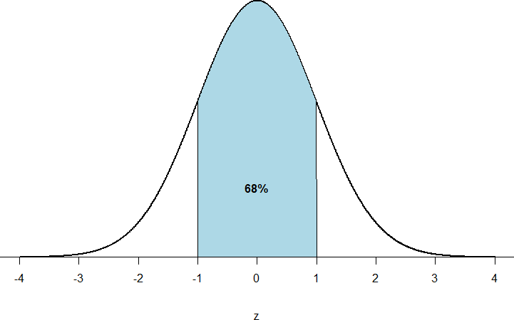
Figure 1: Normal distribution with 68% of z-scores within 1 standard deviation of the mean

We can draw a line through the normal distribution to split it into sections. Take a look at the normal distribution in Figure 2 which has a line drawn through it as z = 1.25. This line creates two sections of the distribution: the smaller section called the tail and the larger section called the body. Differentiating between the body and the tail does not depend on which side of the distribution the line is drawn. All that matters is the relative size of the pieces: the bigger portion is always the body of the distribution.

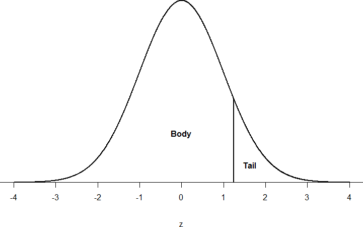
Figure 2. Body and tail of the normal distribution

As you can see, we can break up the normal distribution into three pieces (lower tail, body, and upper tail) as in Figure 1 or into two pieces (body and tail) as in Figure 2. We can then find the proportion of the area in the body and tail based on where the line was drawn (i.e., at what z-score). Mathematically this is done using calculus (don’t worry this is beyond the scope of this course, someone has already done this for you). The exact values are given to you in a Standard Normal Distribution Table, also known as a z-table. Using the values in this table, we can find the area under the normal curve. Many of these tables exist, you will need a z-score to find the area under the curve. Statistical software will calculate the area under the curve for you, which is often called the p-value. This will be discussed in more detail in later chapters.

Probability: The Bigger Picture

The concepts and ideas presented in this chapter are the heart of how inferential statistics work.

To summarize, the probability that an event happens is the number of outcomes that qualify as that event compared to the total number of outcomes. This extends to graphs like a pie chart, where the biggest slices take up more of the area and are therefore more likely to be chosen at random. This idea then brings us back around to our normal distribution, which can also be broken up into regions or areas, each of which are bounded by one or two z-scores and correspond to all z- scores in that region. The probability of randomly getting one of those z-scores in the specified region can then be found on the Standard Normal Distribution Table (aka z-table). Thus, the larger the region, the more likely an event is, and vice versa. Because the tails of the distribution are, by definition, smaller as we go farther out into the tail, the likelihood or probability of finding a result out in the extremes becomes smaller as we will see when we discuss inferential statistics.