5 Measures of Variability
Learning Outcomes
In this chapter, you will learn how to:
- Explain the purpose of measuring variability and differences between scores with high versus low variability.
- Define and calculate measures of variability.
Measures of central tendency (a value around which other scores in the set cluster) and a measure of variability (an indicator of how spread out scores are in a dataset) are often used together to give a description of the data. The terms variability, spread, and dispersion are statistical synonyms, and refer to how spread out a distribution is.
Measures of variability describe the spread of scores in a distribution. The more spread out the scores are, the higher the variability. In Figure 1, the y-axis is frequency and the x-axis represents values for a variable. There are two distributions, labeled as small and large. You can see both are normally distributed (unimodal, symmetrical), and the mean, median, and mode for both fall on the same point. What is different between the two is the variability of the scores. The taller-looking distribution shows a smaller variability while the wider distribution shows a larger variability. For the "small" distribution in Figure 1, the data values are concentrated close to the mean; in the "large" distribution, the data values are more spread out from the mean.
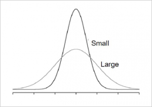 Figure 1. Examples of 2 normal (symmetrical, unimodal) distributions.
Why measure variability?
An important characteristic of any set of data is the variability. Imagine that students in two different sections of statistics take Exam 1 and the mean score in both classrooms is a 75. If that is the only descriptive statistic we report you might assume that both classes are identical - but that is not necessarily true. Let’s examine the scores for each section.
| Section A | Section B |
| Scores = 60, 60, 60, 80, 95, 95
Mean = 75 |
Scores = 69, 72, 73, 75, 76, 85
Mean = 75 |
Table 1. Exam scores for 2 sections of a class.
For Section A very few scores are represented (e.g., 70 and 85) and they are very far from the mean. However, in Section B more scores are represented (6 different scores) and the values are clustered close to the mean. We would say that the spread of scores for Section A is greater than Section B. So, it would be important to calculate the variability for these two sections to compare along with their means to make any sort of informed decision about the two groups.
Just as in the chapter on central tendency where we discussed multiple measures of the center of a distribution of scores, in this chapter we will discuss multiple measures of the variability of a distribution: range, interquartile range, sums of squares, variance, and standard deviation.
Range
The range is the simplest measure of variability and is really easy to calculate. Range is calculated by substracting the smallest score from the largest score in the dataset.
You can see in our statistics course example (Table 1) that Section A scores have a range of 35 (95-60=35) and Section B scores have a range of 16 (85-69=16). That means all the other scores are not included; thus, range may give a biased description of the data. The simplicity of calculating range is appealing but it can be a very unreliable measure of variability.
Let’s take a few examples. What is the range of the following group of numbers: 10, 2, 5, 6, 7, 3, 4? Well, the highest number is 10, and the lowest number is 2, so 10 - 2 = 8. The range is 8. Let’s take another example. Here’s a dataset with 10 numbers: 99, 45, 23, 67, 45, 91, 82, 78, 62, 51. What is the range? The highest number is 99 and the lowest number is 23, so 99 - 23 equals 76; the range is 76. Again, the problem with using range is that it is extremely sensitive to outliers, and one number far away from the rest of the data will greatly alter the value of the range. For example, in the set of numbers 1, 3, 4, 4, 5, 8, and 9, the range is 8 (9 – 1). However, if we add a single person whose score is nowhere close to the rest of the scores, say, 20, the range more than doubles from 8 to 19.
Interquartile Range
A special take on range, is to identify values in terms of quartiles of the distribution (remember chapter 3 with box plots). The interquartile range (IQR) is the range of the middle 50% of the scores in a distribution and is sometimes used to communicate where the bulk of the data in the distribution are located. It is computed as follows: IQR = 75th percentile - 25th percentile.
The Mean Needed to Further Examine Variability
Variability can also be defined in terms of how close the scores in the distribution are to the middle of the distribution. Using the mean as the measure of the middle of the distribution, we can see how far, on average, each data point is from the middle. Remember that the mean is the point on which a distribution would balance. We can examine spread by identifying how far each value is from the mean. This is known as the deviation from the mean (or differences or distances from the mean).
Let's revisit an example from chapter 4 (Figure 2). We had a set of 5 numbers: 2, 3, 4, 9, and 16 with a mean of 6.8.
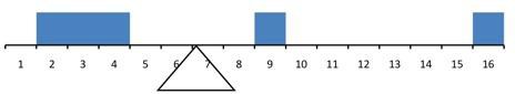
Figure 2. The distribution balances at the mean of 6.8.
In Table 2, the value is represented as X, the column "deviation from the mean or 𝑋 − M” contains deviations (how far each score deviates from the mean), here calculated as the score minus 6.8.
|
Value (X) |
(X - M) |
Deviation from the Mean (X - M) |
|
2 |
2-6.8 |
-4.8 |
|
3 |
3-6.8 |
-3.8 |
|
4 |
4-6.8 |
-2.8 |
|
9 |
9-6.8 |
2.2 |
| 16 |
16-6.8 |
9.2 |
|
Total (Σ ) |
|
0 |
Table 2. Deviations of the numbers 2, 3, 4, 9, and 16 from their mean of 6.8.
We are trying to get to a measure of spread or variability around the mean. However, when we sum up the deviation scores calculated in Table 2, we see that they add up to zero. This occurs because the mean is the balance point, and half of the deviations or distance totals are negative and half are positive. So, we must find a way to get this measure of spread without these negative numbers. Some will look at taking the absolute values of the deviation scores, creating an mean absolute deviation. But this is not what we typically use. Let's look at our more typical measures of variability.
Sums of Squares
For us to get to a value that would represent the variability, we will add another step from calculating the deviation of the mean scores. You can see in Table 3 there is now a new column, the squared deviations column. The column “(𝑋 − M)2” has the “Squared Deviations” and is simply the previous column squared. Notice that this too gets rid of the negative values.
|
Value (X) |
Deviation from the Mean (X - M) |
Squared Deviations (X-M)2 |
|
2 |
-4.8 | (-4.8)x(-4.8)=23.04 |
|
3 |
-3.8 | (-3.8)x(-3.8)=14.44 |
|
4 |
-2.8 | (-2.8)x(-2.8)=7.84 |
|
9 |
2.2 | (2.2)x(2.2)=4.84 |
| 16 | 9.2 | (9.2)x(9.2)=84.64 |
|
Total (Σ ) |
0 | 134.8 (←Sum of Squares/SS) |
Table 3. Adding on a squared deviations column to create "sum of squares" or SS
Here is another example of calculating SS with 20 data points where the mean = 7 (140/20):
| X | f | f(X) | X − M | f(X-M) | (X − M)2 | f(X-M)2 |
|
9 |
3 |
3x9=27 |
2 |
3x2=6 |
4 |
3x4=12 |
|
8 |
4 |
4x8=32 |
1 |
4x1=4 |
1 |
4x1=4 |
|
7 |
5 |
5x7=35 |
0 |
5x0=0 |
0 |
5x0=0 |
|
6 |
6 | 6x6=36 | -1 |
6x(-1)=-6 |
1 |
6x1=6 |
|
5 |
2 | 2x5=10 | -2 |
2x(-2)=-4 |
4 |
2x4=8 |
|
total (Σ ) |
20 |
140 |
|
0 |
|
SS = 30 |
Table 4. Calculations for Sum of Squares with definitional formula.
There are a few things to note about how Table 4 is formatted, as this is the format you will use to calculate sums of squares (SS), and soon variance and standard deviation. The raw data scores (X) are always placed in the left-most column. The second column (f) represents the number of times (or frequency) of each of these scores. The third column is calculated by multiplying the first two columns. These second and third columns are then summed at the bottom to facilitate calculating the mean (simply divide the total of the f(X) column by the total of the f column). Once you have the mean, you can easily work your way down the next column calculating the deviation scores. Note that you must multiply each new column by the frequency column before summing the column. The f(X-M) column is also summed and has a very important property: it will always sum to 0 (or close to zero if you have rounding error due to many decimal places). This step is used as a check on your math to make sure you haven’t made a mistake. If this column sums to 0, you can move on to filling in the column of squared deviations. This column is multiplied by the frequency column and then summed as well and has its own name: the Sum of Squares (abbreviated as SS and given the definitional formula ∑(X−M)2). As we will see, the Sum of Squares appears again and again in different formulas – it is a very important value, and this table makes it simple to calculate without error.
There is another method by which you can calculate the Sums of Squares (SS) called the computational formula that we will show you next. Ultimately you can choose to use either formula. This second method results in less chance for rounding error but isn't more correct than the one above. To use the computational method, first you complete the calculations outlined in Table 5 below.
| X | f | f(X) | X2 | f(X2) |
|
9 |
3 |
3x9=27 |
9x9=81 |
3x81=243 |
|
8 |
4 |
4x8=32 |
8x8=64 |
4x64=256 |
|
7 |
5 |
5x7=35 |
7x7=49 |
5x49=245 |
|
6 |
6 | 6x6=36 | 6x6=36 |
6x36=216 |
|
5 |
2 | 2x5=10 | 5x5=25 |
2x25=50 |
|
total (Σ ) |
20 |
140 |
|
1,010 |
Table 5. Calculations for Sum of Squares with computational formula.
To then calculate SS using the computational formula, you have to do some calculations outside of the table using the equation below.
[latex]SS=\Sigma{X^2}-\frac{(\Sigma X)^2}{N}[/latex]
In terms of the column headers in Table 5, this computational formula for SS looks like this:
[latex]SS=f(X^2)-\frac{(f(X))^2}{f}=1010-\frac{140^2}{20}=30[/latex]
Sums of Squares (SS)
Sums of squares (SS), short for sum of the squared deviations from the mean, can be calculated two ways: using the definitional formula or the computation formula. The definitional formula is called that because the formula follows the definition. It is the sum (Σ) of the squared deviations (X-M)2. While the computational formula does not look like the definition. However, either route will get you to the same answer minus some rounding error differences. Whichever formula you choose to use, remember that they both start with the creation of a frequency distribution table.
Definitional Formula:
[latex]SS=\Sigma{(X-M)^2}[/latex]
Computational Formula:
[latex]SS=\Sigma{X^2}-\frac{(\Sigma X)^2}{N}[/latex]
Example from Table 3. Table 3 demonstrates the use of the definitional formula for a small dataset. We can apply the computational formula for that same small dataset without a frequency table.
Definitional Formula:
[latex]SS=\Sigma{(X-M)^2}=(23.04+14.44+7.84+4.84+84.64)=134.8[/latex]
Computational Formula:
[latex]SS=\Sigma{X^2}-\frac{(\Sigma X)^2}{N}=(2^2+3^2+4^2+9^2+16^2)-\frac{(2+3+4+9+16)^2}{5}[/latex]
[latex]SS=366-\frac{34^2}{5}=366-\frac{1156}{5}=366-231.2=134.8[/latex]
Variance
Now that we have the Sum of Squares calculated, we can use it to compute our formal measure of average deviation from the mean, the variance. Informally, it measures how far a set of (random) numbers are spread out from their average value. The variance is defined as the average squared deviation of the scores from their mean. The mathematical definition of the variance is the sum of the squared deviations (distances) of each score from the mean divided by the number of scores in the dataset. Remember that we square the deviation scores because, as we saw in the Sum of Squares table, the sum of raw deviations is always 0, and there’s nothing we can do mathematically without changing that.
Variance (Population)
The population parameter for variance is σ2 (pronounced “sigma-squared”) and is calculated as:
[latex]\sigma^2=\frac{SS}{N}[/latex]
Example from Table 3. If we assume that the values in Table 3 represent the full population, then we can take our value of SS and divide it by N to get our population variance:
[latex]\sigma^2=\frac{SS}{N}=\frac{134.8}{5}=26.96[/latex]
Example from Table 4. If we assume that the values in Table 4 represent the full population, then we can take our value of SS and divide it by N to get our population variance:
[latex]\sigma^2=\frac{SS}{N}=\frac{30}{20}=1.50[/latex]
So, on average, scores in the population from our quiz example in Table 4 are 1.5 squared units (or points because the quiz is measured as points) away from the mean. While measured variability in terms of squared units isn't necessarily meaningful, as we will see in future chapters, variance plays a central role in inferential statistics.
Variance (Sample)
The sample statistic used to estimate the variance is s2 (“s-squared”):
[latex]s^2=\frac{SS}{n-1}[/latex]
Note: the sum of squared deviations is abbreviated as SS and the degrees of freedom is abbreviated as df. The shorthand for sample variance is SS/df.
[latex]s^2=\frac{SS}{n-1}=\frac{SS}{df}[/latex]
Example from Table 3. If we assume that the values in Table 3 represent the sample, then we can take our value of SS and divide it by df (or n-1) to get our sample variance:
[latex]s^2=\frac{SS}{df}=\frac{134.8}{5-1}=33.70[/latex]
Example from Table 4. If we assume that the values in Table 4 represent the sample, then we can take our value of SS and divide it by df (or n-1) to get our sample variance:
[latex]s^2=\frac{SS}{df}=\frac{30}{20-1}=1.58[/latex]
Notice that the sample variance values are slightly larger than the one we calculated when we assumed these scores were the full population. This is because our value in the denominator is slightly smaller, making the final value larger. In general, as your sample size, n, gets bigger, the better it represents the population and thus the closer the sample variance will be to the population variance. Mathematically speaking, as the n gets bigger, the effect of subtracting 1 becomes less and less.
Standard Deviation
The standard deviation is simply the square root of the variance. This is a useful and interpretable statistic because taking the square root of the variance (recalling that variance is the average squared difference) puts the standard deviation back into the original units of the measure we used. When reporting descriptive statistics in a study, if researchers report a mean they virtually always report the corresponding standard deviation. Additionally, when compared to the range, the standard deviation is a much more robust (a term used by statisticians to mean resilient or resistant to outliers) measure of variability. Standard deviation is therefore the most commonly used measure of variability.
The population parameter for standard deviation is σ (“sigma”). Notice it is the same symbol as variance but without the "squared" part. Thus, standard deviation is simply the square root of the variance parameter σ2 (on occasion, the symbols work out nicely that way).
Standard Deviation (Population)
Population standard deviation is given as σ ("sigma").
[latex]\sigma=\sqrt{\sigma^2}=\sqrt{\frac{SS}{N}}[/latex]
Example from Table 3. If we assume that the values in Table 3 represent the full population, then we can take our value of SS and divide it by N to get our population standard deviation:
[latex]\sigma=\sqrt{\sigma^2}=\sqrt{\frac{SS}{N}}=\sqrt{\frac{134.8}{5}}=\sqrt{26.96}=5.19[/latex]
Example from Table 4. If we assume that the values in Table 4 represent the full population, then we can take our value of SS and divide it by N to get our population standard deviation:
[latex]\sigma=\sqrt{\sigma^2}=\sqrt{\frac{SS}{N}}=\sqrt{\frac{30}{20}}=\sqrt{1.50}=1.22[/latex]
The sample statistic follows the same conventions and is given as s. It is simply the square root of the sample variance.
Standard Deviation (Sample)
Sample standard deviation is given as s (just "s").
[latex]s=\sqrt{s^2}=\sqrt{\frac{SS}{df}}=\sqrt{\frac{SS}{n-1}}[/latex]
Example from Table 3. If we assume that the values in Table 3 represent the sample, then we can take our value of SS and divide it by df (or n-1) to get our sample standard deviation:
[latex]s=\sqrt{s^2}=\sqrt{\frac{SS}{df}}=\sqrt{\frac{134.8}{5-1}}=\sqrt{33.70}=5.81[/latex]
Example from Table 4. If we assume that the values in Table 4 represent the sample, then we can take our value of SS and divide it by df (or n-1) to get our sample standard deviation:
[latex]s=\sqrt{s^2}=\sqrt{\frac{SS}{df}}=\sqrt{\frac{30}{20-1}}=\sqrt{1.58}=1.26[/latex]
Interestingly, if we were writing these descriptive statistics in a paper, we wouldn't use σ or s. For example, let's imagine the data from Table 3 represented the ages of five kids in a family, and you wanted to write a sentence that described this distribution. It could be written as such in APA style.
Family A completed the American Community Survey resulting in an average age for their children (n = 5, M = 6.8, SD = 5.81).
Notice that the abbreviation SD is used for Standard Deviation when writing up the results of your data analysis. Also, notice that descriptive statistics go inside parentheses.
The Normal Distribution and Standard Deviation
The standard deviation is an especially useful measure of variability when the distribution is normal or approximately normal because the proportion of the distribution within a given number of standard deviations from the mean can be calculated. By definition, the normal distribution has certain characteristics.
For a normal distribution,
- The shape of the distribution is symmetrical (no skew).
- Approximately 68% of the data is within one standard deviation of the mean.
- Approximately 95% of the data is within two standard deviations of the mean.
- More than 99% of the data is within three standard deviations of the mean.
This is known as the Empirical Rule or the 68-95-99 Rule, as shown in Figure 3.
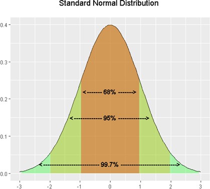
Figure 3. Percentages of the normal distribution showing the 68-95-99 rule.
For example, if you had a normal distribution with a mean of 50 and a standard deviation of 10, then 68% of the distribution would be between 40 and 60 (i.e., 50 - 10 = 40 and 50 +10 = 60). Similarly, about 95% of the distribution would be between 30 and 70 (i.e., 50 - 2 x 10 = 30 and 50 + 2 x 10 = 70). And, about 99% would be between 20 and 80 (i.e., 50 - 3 x 10 = 20 and 50 + 3 x 10 = 80).
Figure 4 shows two normal distributions. The red distribution has a mean of 40 and a standard deviation of 5; the blue distribution has a mean of 60 and a standard deviation of 10. For the red distribution, 68% of the distribution is between 45 and 55; for the blue distribution, 68% is between 50 and 70. Notice that as the standard deviation gets smaller, the distribution becomes much narrower and taller, regardless of where the center of the distribution (mean) is. Figure 5 presents several more examples of this effect.
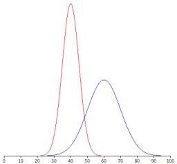
Figure 4. Normal distributions with standard deviations of 5 and 10.
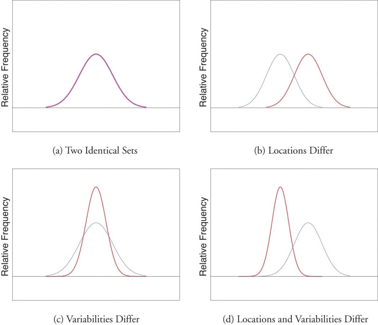
Figure 5. Differences between two datasets.
The image below represents IQ scores as measured by the Wechsler Intelligence test and has a µ = 100 and σ = 15. This means that about 68% of the scores are between 85 and 115 and that 95% of the scores are between 70 and 130.
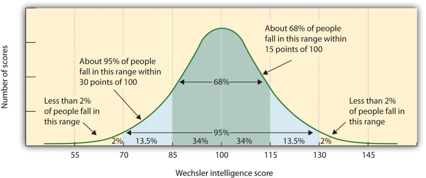
Figure 6. Weshcler IQ Score distribution. Photo credit
A data value that is two standard deviations from the mean is just on the borderline for what many statisticians would consider to be far from the mean (outside or non-adjacent values from chapter 3), and they would define outside two standard deviations as an outlier (extreme score). Some researchers may define an outlier as greater than 3 standard deviations from the mean. In general, the shape of the distribution of the data affects how much of the data is further away than two standard deviations.
Recap
While range is a very simple measure of variability, it isn't very robust. Thus, it is highly affected by outliers and should be used with caution.
Recall that the symbol and equation (specifically, the denominator) for the variance changes depending on whether the statistic is referring to a sample or a population. Although the variance is itself a measure of variability, it generally plays a larger role in inferential statistics than in descriptive statistics.
The standard deviation is the most commonly used measure of variability because it includes all the scores of the data set in the calculation, and it is reported in the original units of measurement. It tells us the average (or standard) distance of each score from the mean of the distribution.
The standard deviation is always positive or zero. The standard deviation is small when the data are all concentrated close to the mean, exhibiting little variation or spread. The standard deviation is larger when the data values are more spread out from the mean, exhibiting more variation.
It is important to note that the Empirical Rule or the 68-95-99 rule only applies when the shape of the distribution of the data is normal (bell-shaped and symmetric).
Factors Affecting Variability
Before we close out the chapter, we wanted to make you aware that there are a couple of things that can impact the spread of scores.
Extreme Scores. Range is affected most by extreme scores or outliers but standard deviation and variance are also affected by extremes because they are based on squared deviations. One extreme score can have a disproportionate effect on the overall statistic or parameter. (And, remember, the mean, which is used in the calculation of variance and standard deviation, is also affected by outliers.)
Sample size. Increased sample size is associated with an increase in range because of the potential to increase or decrease the minimum or maximum values in a dataset. However, increasing sample size is good for variance and standard deviation because it helps ensure better representation of population variance and standard deviation.
A statistical measures that identifies a single score (usually a central value) to serve as a representative for the entire group.
the degree to which members of a group or population or scores in a dataset differ from each other
The distance from the upper real limit of the highest score to the lower real limit of the lowest score; the total distance from the absolute highest point to the lowest point in the distribution.
The range of the middle 50% of the scores in a distribution and is sometimes used to communicate where the bulk of the data in the distribution are located.
The sum of the squared deviation scores.
The average squared deviation of the scores from the mean.
Degrees of freedom = df = n – 1, measures the number of scores that are free to vary when computing SS for sample data. The value of df also describes how well a t statistic estimates a z-score. (as discussed in Unit 3).
a measure of the variability within a sample, indicating how narrowly or broadly they deviate from the mean.
A distribution where the left-hand side is a mirror image of the right-hand side. Also known as symmetrical distribution.
68% of all scores within 1 standard deviation of the mean; 95% of all scores within 2 standard deviations of the mean; 99% of all scores within 3 standard deviations of the mean. Also known as the 68-95-99 Rule.
Observation or data point that does not fit the pattern of the rest of the data. Sometimes called an extreme value.
