3 Describing Data
Learning outcomes
In this chapter, you will learn how to:
- Identify different types of graphs and when we would use them based on the type of data.
- Create a frequency distribution table.
- Differentiate between different types of frequency graphs.
- Identify the shape of a distribution in a frequency graph.
Statistics that are used to organize and summarize the information so that the researcher can see what happened during the research study and can also communicate the results to others are called descriptive statistics. Let us assume that the data are quantitative and consist of scores on one or more variables for each of several study participants. Although in most cases the primary research question will be about one or more statistical relationships between variables, it is also important to describe each variable individually. We will look at some of the most common techniques for describing single variables including:
- Frequency distributions and graphs
- Measures of Central Tendency
- Measures of Variability
The first step in understanding data is using tables, charts, graphs, plots, and other visual tools to see what our data look like. This is known as data visualization.
Data Visualization
On January 28, 1986, the Space Shuttle Challenger exploded 73 seconds after takeoff, killing all 7 of the astronauts on board. As when any such disaster occurs, there was an official investigation into the cause of the accident, which found that an O-ring connecting two sections of the solid rocket booster leaked, resulting in failure of the joint and explosion of the large liquid fuel tank (see figure 1).[1]
![An image of the solid rocket booster leaking fuel, seconds before the explosion. The small flame visible on the side of the rocket is the site of the O-ring failure. By NASA (Great Images in NASA Description) [Public domain], via Wikimedia Commons](https://open.ocolearnok.org/app/uploads/sites/78/2021/06/file9.jpg)
The investigation found that many aspects of the NASA decision-making process were flawed, and focused in particular on a meeting between NASA staff and engineers from Morton Thiokol, a contractor who built the solid rocket boosters. These engineers were particularly concerned because the temperatures were forecast to be very cold on the morning of the launch, and they had data from previous launches showing that performance of the O-rings was compromised at lower temperatures. In a meeting on the evening before the launch, the engineers presented their data to the NASA managers, but were unable to convince them to postpone the launch. Their evidence was a set of hand-written slides showing numbers from various past launches.
The visualization expert Edward Tufte has argued that with a proper presentation of all of the data, the engineers could have been much more persuasive. In particular, they could have shown a figure like the one in Figure 1, which highlights two important facts. First, it shows that the amount of O-ring damage (defined by the amount of erosion and soot found outside the rings after the solid rocket boosters were retrieved from the ocean in previous flights) was closely related to the temperature at takeoff. Second, it shows that the range of forecasted temperatures for the morning of January 28 (shown in the shaded area) was well outside of the range of all previous launches. While we can’t know for sure, it seems at least plausible that this could have been more persuasive.
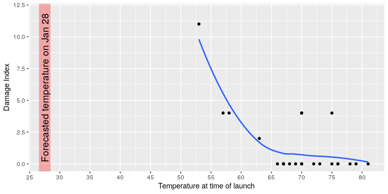
Figure 1. A replotting of Tufte’s damage index data. The line shows the trend in the data, and the shaded patch shows the projected temperatures for the morning of the launch.
Graphing Qualitative & Quantitative Variables
We’ll learn some general lessons about how to graph data that fall into a small number of categories. A later section will consider how to graph numerical data in which each observation is represented by a number in some range. Qualitative variables can be summarized by frequency (how often) and researchers can then use frequency tables and bar charts to show frequencies for categorized responses, but we are limited in graphing them due to the data not being numerically based. The key point about the qualitative data is they do not come with a pre-established ordering (the way numbers are ordered).
Here we will focus on quantitative variables. Quantitative data, such as a person’s weight, are naturally ordered with respect to people of different weights. Often we wish to know if there are any scores that might look a bit out of place. A frequency distribution is a way to take a disorganized set of scores and place them in order from highest to lowest and at the same time grouping everyone with the same score. Frequency distributions can help researchers identify outliers. An outlier is an observation of data that does not fit the rest of the data. An outlier is sometimes called an extreme value. When you graph an outlier, it will appear not to fit the pattern of the graph. Some outliers are due to mistakes (for example, writing down 50 instead of 500) while others may indicate that something unusual is happening.
Frequency Tables
All of the graphical methods shown in this section are derived from frequency tables. For example, a survey asked individuals what type of computer they currently owned. Table 1 shows a frequency table for the results of the study; it shows the frequencies of the various response categories. It also shows the relative frequencies, which are the proportion of responses in each category. For example, the relative frequency for “none” of 0.17 = 85/500.
|
Previous Ownership |
Frequency |
Relative Frequency |
|
None |
85 |
0.17 |
|
Windows |
60 |
0.12 |
|
iMac |
355 |
0.71 |
|
Total |
500 |
1 |
Table 1. Frequency Table for the iMac Data.
Below is a table (Table 2) showing a hypothetical distribution of scores on the Rosenberg Self-Esteem Scale for a sample of 40 college students. The Rosenburg Self-Esteem Scale is one way to operationalize (define) self-esteem in a quantitative way. Participants rate each of the 10-items from strongly disagree to strongly agree. All items are then scored yielding an overall self-esteem score that would be a numerical value to represent one’s self-esteem.
- The first column (on the left) lists the values (the possible scores on the Rosenberg scale) of the variable.
- The second column (on the right) lists the frequency (number of times each occurs in the data) of each score.
| Self-Esteem Scores | Frequency |
| 24 | 3 |
| 23 | 5 |
| 22 | 10 |
| 21 | 8 |
| 20 | 5 |
| 19 | 3 |
| 18 | 3 |
| 17 | 0 |
| 16 | 2 |
| 15 | 1 |
Table 2. Frequency Table for Rosenburg Self-Esteem Scale Scores.
Table 2 shows that there were three students who had self-esteem scores of 24, five who had self-esteem scores of 23, and so on. From a frequency table like this, one can quickly see several important aspects of a distribution, including the range of scores (from 15 to 24), the most and least common scores (22 and 17, respectively), and any extreme scores that stand out from the rest.
Considerations
There are a few other points worth noting about frequency tables. First, the levels listed in the first column usually go from the highest at the top to the lowest at the bottom, and they usually do not extend beyond the highest and lowest scores in the data. For example, although scores on the Rosenberg scale can vary from a high of 30 to a low of 0, the frequency table only includes levels from 24 to 15 because that range includes all the scores in this particular data set. All scores within the dataset must be presented. For example, no one received a score of 17 on the Rosenberg Self-esteem scale; it is still represented in the table.
Additionally, when there are many different scores across a wide range of values, it is often better to create a grouped frequency table, in which the first column lists ranges of values and the second column lists the frequency of scores in each range. In a grouped frequency table, the ranges must all be of equal width, and there are usually between five and 15 of them (see Table 3 below for this same data in a grouped frequency table version).
| Self-Esteem Scores | Frequency |
| 26 – 30 | 0 |
| 21 – 25 | 26 |
| 16 -20 | 13 |
| 11 – 15 | 1 |
| 6 -10 | 0 |
| 1 -5 | 0 |
Table 3. Grouped Frequency Table for Rosenburg Self-Esteem Scale Scores.
Finally, frequency tables can also be used for categorical variables, in which case the levels are category labels. The order of the category labels is somewhat arbitrary, but they are often listed from the most frequent at the top to the least frequent at the bottom. Table 4 shows an example for majors where majors is a categorical (nominal) variable and they are listed in no particular order.
| Majors | Frequency |
| Business | 30 |
| Psychology | 50 |
| Nursing | 102 |
| Nutritional Sciences | 10 |
| Communications | 5 |
| English | 3 |
| Computer Science | 13 |
Graphs
A graph is a visual tool that helps you learn about the shape or distribution of a sample or population. A graph can be a more effective way of presenting data than a list or table of numbers because we can see where data clusters and where there are only a few data values.
Some of the types of graphs that are used to summarize and organize data are the scatterplot, bar graph, histogram, stem-and-leaf plot, line graph, frequency polygon, pie chart, and box plot. In this section, we will briefly look at bar graphs, histograms, frequency polygons, and box plots.
Bar graphs
Bar graphs are used to represent frequencies of discrete categories. Bar graphs are appropriate for qualitative data (categorical variables) and other discrete variables that use a nominal or ordinal scale of measurement. A bar graph of the iMac purchases is shown in Figure 2. Frequencies are shown on the y-axis (the vertical axis) and the type of computer previously owned is shown on the x-axis (the horizontal axis). (Typically, the y-axis shows the number of observations in each category.)
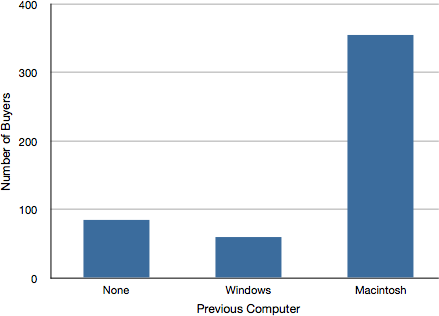
Figure 2. Bar graph of iMac purchases as a function of previous computer ownership.
Comparing Distributions
Often we need to compare the results of different surveys, or of different conditions within the same overall survey. In this case, we are comparing the “distributions” of responses between the surveys or conditions. Bar graphs are excellent for illustrating differences between two distributions between discrete variables. Figure 4 shows the number of people playing card games at the Yahoo website on a Sunday and on a Wednesday in the spring of 2001. We see that there were more players overall on Wednesday compared to Sunday. The number of people playing Pinochle was nonetheless the same on these two days. In contrast, there were about twice as many people playing hearts on Wednesday as on Sunday. Facts like these emerge clearly from a well-designed bar graph.
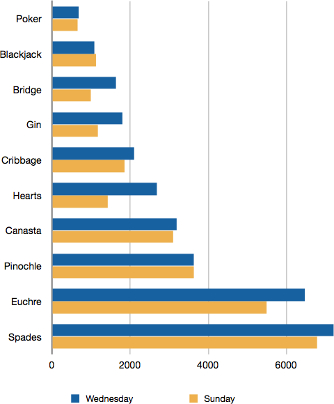 Figure 3. A bar graph of the number of people playing different card games on Sunday and Wednesday.
The bars in Figure 3 are oriented horizontally rather than vertically. The horizontal format is useful when you have many categories because there is more room for the category labels.
Some graphical mistakes to avoid with bar graphs
Don’t get fancy! People sometimes add features to graphs that don’t help to convey their information. See the examples below as things not to do! Three-dimensional figures are less clear than 2-d. Further, don’t get creative as shown below! Use plain bars, as tempting as it is to substitute meaningful images. The MacIntosh is out of proportion to the None and Windows categories. Edward Tufte coined the term “lie factor” to refer to the ratio of the size of the effect shown in a graph to the size of the effect shown in the data. If a graphic has a lie factor near 1, then it is appropriately representing the data, whereas lie factors far from one reflect a distortion of the underlying data. The computer monitor bar figure has a lie factor of about 8! He suggests that lie factors greater than 1.05 or less than 0.95 produce unacceptable distortion-so just keep it simple with plain bars!
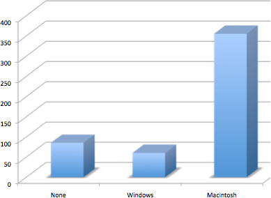
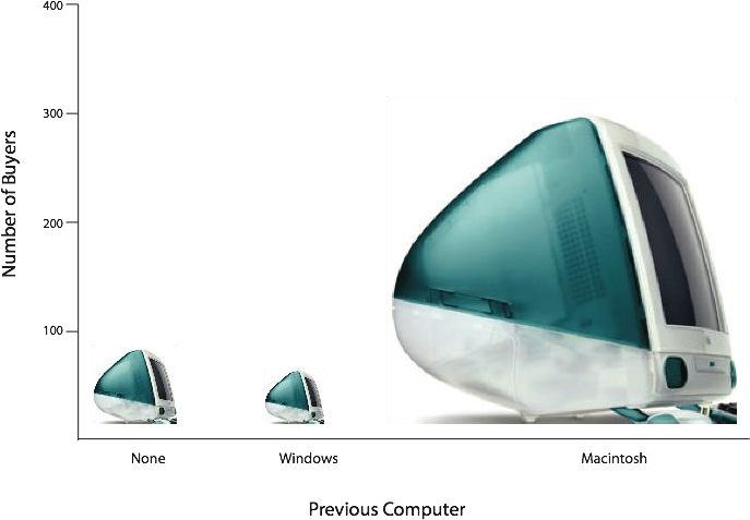
Figures 4 & 5. A three-dimensional version of Figure 2 and a redrawing of Figure 2 with disproportionate bars.
In Figure 6 below (created using Microsoft Excel) plots the relative popularity of different religions in the United States. There are at least three things wrong with this figure. Can you identify them?
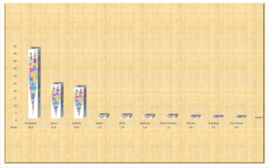
Figure 6. A bad bar graph
Did you figure out what is wrong?
- It has graphics overlaid on each of the bars that have nothing to do with the actual data
- It has a distracting background texture
- It uses three-dimensional bars, which distort the data
Another distortion in bar graphs results from setting the baseline to a value other than zero. The baseline is the bottom of the y-axis, representing the least number of cases that could have occurred in a category. Normally, but not always, this number should be zero. Figure 8 shows the iMac data with a baseline of 50. Once again, the differences in areas suggests a different story than the true differences in percentages. The number of Windows-switchers seems minuscule compared to its true value of 12%.
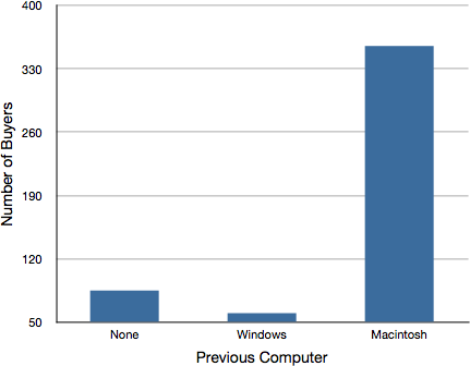
Figure 7. A redrawing of Figure 2 with a baseline of 50.
Finally, we note that it is a serious mistake to use a line graph when the x-axis contains merely qualitative (or categorical) variables. A line graph is essentially a bar graph with the tops of the bars represented by points joined by lines. Figure 8 inappropriately shows a line graph of the card game data from Yahoo. The drawback to Figure 8 is that it gives the false impression that the games are naturally ordered (on a continuum) in a numerical way when, in fact, they are ordered alphabetically. If the x-axis represented the days of the week, representing time which is on a continuum, a line graph would be more appropriate.
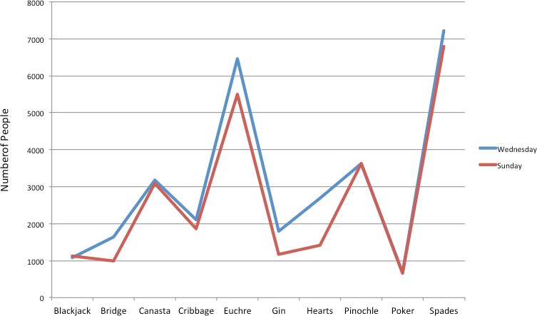
Figure 8. A line graph used inappropriately to depict the number of people playing different card games on Sunday and Wednesday.
Recap
Bar graphs can be effective methods of portraying qualitative data. Bar graphs are better when there are more than just a few categories and for comparing two or more distributions. Finally, be careful to avoid creating misleading graphs.
Graphing Quantitative Variables
As discussed in the section on variables in Chapter 2, quantitative variables are variables measured on a numeric scale. Height, weight, response time, subjective rating of pain, temperature, and score on an exam are all examples of quantitative variables. Quantitative variables are distinguished from categorical (sometimes called qualitative) variables such as favorite color, religion, city of birth, favorite sport in which there is no ordering or measuring involved. There are many types of graphs that can be used to portray distributions of quantitative variables including but not limited to: histograms, frequency polygons, box plots, line graphs, and scatter plots (discussed in a different chapter). Let’s explore some of these graphs now.
Histograms
A histogram is a graphic version of a frequency distribution for continuous (i.e., interval and ratio) variables. It helps to display the shape of a distribution. The graph consists of bars of equal width drawn adjacent to each other. The horizontal axis (x-axis) is labeled with what the data represents (for instance, distance from your home to school). The vertical axis (y-axis) represents the frequency, relative frequency, percent frequency, or probability.
As with a bar graph, before we can create a histogram, we must create a frequency distribution table. However, the data for a histogram is often much more complex than the data for a bar graph. Here is an example.
If we wanted to create a frequency distribution of 642 students’ scores on a psychology test, that would be a big frequency table. Imagine that the test consists of 197 items each graded as “correct” or “incorrect,” and that the students’ scores ranged from 46 to 167. If you created a simple frequency table would be too big, containing over 100 rows. As you might recall, an ideal frequency distribution table has between 5 and 15 rows. So, to simplify the table, we could group scores together into “intervals” more officially known as class intervals. A basic rule for grouping data is to make sure each group (or interval) has the same width or size. Let’s pick an interval width of 10 for our example. Another rule is to make sure you ensure that the lowest interval or category includes your lowest value (or test score) and the highest interval or category includes your highest value (or test score) to make sure all scores are included. Then, in order to create our histogram, we need to identify the “upper limit” and “lower limit” of our class intervals. This is where the bars on our histograms meet. See Table 5 for our example data and Figure 9 for the histogram of this data.
|
Interval |
Interval’s Lower Limit |
Interval’s Upper Limit |
Interval Frequency |
| 40 – 49 | 39.5 | 49.5 | 3 |
| 50 – 59 | 49.5 | 59.5 | 10 |
| 60 – 69 | 59.5 | 69.5 | 53 |
| 70 – 79 | 69.5 | 79.5 | 107 |
| 80 – 89 | 79.5 | 89.5 | 147 |
| 90 – 99 | 89.5 | 99.5 | 130 |
| 100 – 109 | 99.5 | 109.5 | 78 |
| 110 – 119 | 109.5 | 119.5 | 59 |
| 120 – 129 | 119.5 | 129.5 | 36 |
| 130 – 139 | 129.5 | 139.5 | 11 |
| 140 – 149 | 139.5 | 149.5 | 6 |
| 150 – 159 | 149.5 | 159.5 | 1 |
| 160 – 169 | 159.5 | 169.5 | 1 |
Table 5. Grouped Frequency Distribution of Psychology Test Scores
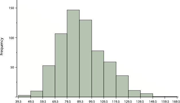
Figure 9. Histogram of scores on a psychology test.
The histogram makes it plain that most of the scores are in the middle of the distribution, with fewer scores in the extremes. You can also see that the distribution is not symmetric: the scores extend to the right farther than they do to the left. The distribution is therefore said to be skewed. (We’ll have more to say about shapes of distributions a little later in the chapter).
Histograms can be based on relative frequencies instead of actual frequencies. Histograms based on relative frequencies show the proportion of scores in each interval rather than the number of scores. In this case, the y-axis runs from 0 to 1 (or somewhere in between if there are no extreme proportions). You can change a histogram based on frequencies to one based on relative frequencies by (a) dividing each class frequency by the total number of observations, and then (b) plotting the quotients on the y-axis (labeled as Relative Frequency).
There is more to be said about the widths of the class intervals, sometimes called bin widths. Your choice of bin width determines the number of class intervals. Most statistical software will allow you to change the bin width for your histograms. This decision, along with the choice of starting point for the first interval, affects the shape of the histogram. The best advice is to experiment with different choices of width, and to choose a histogram according to how well it communicates the shape of the distribution.
Frequency Polygons
Frequency polygons are another graphical device for understanding the shapes of distributions. They serve the same purpose as histograms, but are especially helpful for comparing sets of data. Frequency polygons are also a good choice for displaying cumulative frequency distributions.
To create a frequency polygon, start just as for histograms, by choosing a class interval. Then draw an x-axis representing the values of the scores in your data. Mark the middle of each class interval with a tick mark, and label it with the middle value represented by the class. Draw the y-axis to indicate the frequency of each class. Place a point in the middle of each class interval at the height corresponding to its frequency. Finally, connect the points. You should include one class interval below the lowest value in your data and one above the highest value. The graph will then touch the X-axis on both sides.
A frequency polygon for 642 psychology test scores shown in Figure 10 was constructed from the frequency table shown in Table 5.
|
Lower Limit |
Upper Limit |
Count |
Cumulative Count |
|
29.5 |
39.5 |
0 |
0 |
|
39.5 |
49.5 |
3 |
3 |
|
49.5 |
59.5 |
10 |
13 |
|
59.5 |
69.5 |
53 |
66 |
|
69.5 |
79.5 |
107 |
173 |
|
79.5 |
89.5 |
147 |
320 |
|
89.5 |
99.5 |
130 |
450 |
|
99.5 |
109.5 |
78 |
528 |
|
109.5 |
119.5 |
59 |
587 |
|
119.5 |
129.5 |
36 |
623 |
|
129.5 |
139.5 |
11 |
634 |
|
139.5 |
149.5 |
6 |
640 |
|
149.5 |
159.5 |
1 |
641 |
|
159.5 |
169.5 |
1 |
642 |
|
169.5 |
170.5 |
0 |
642 |
Table 5. Frequency Distribution of Psychology Test Scores
The first label on the X-axis is 35. This represents an interval extending from 29.5 to 39.5. Since the lowest test score is 46, this interval has a frequency of 0. The point labeled 45 represents the interval from 39.5 to 49.5. There are three scores in this interval. There are 147 scores in the interval that surrounds 85.
You can easily discern the shape of the distribution from Figure 10. Most of the scores are between 65 and 115. It is clear that the distribution is not symmetric inasmuch as good scores (to the right) trail off more gradually than poor scores (to the left). We call this skew and we will study shapes of distributions more systematically later in this chapter.
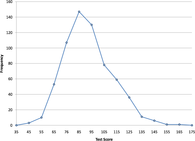
Figure 10. Frequency polygon for the psychology test scores.
A cumulative frequency polygon for the same test scores is shown in Figure 11. The graph is the same as before except that the Y value for each point is the number of students in the corresponding class interval plus all numbers in lower intervals. For example, there are no scores in the interval labeled “35,” three in the interval “45,” and 10 in the interval “55.” Therefore, the Y value corresponding to “55” is 13. Since 642 students took the test, the cumulative frequency for the last interval is 642.
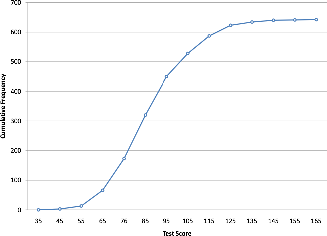
Figure 11. Cumulative frequency polygon for the psychology test scores.
Comparing Distributions with Frequency Polygons
Frequency polygons are useful for comparing distributions. This is achieved by overlaying the frequency polygons drawn for different data sets. Figure 12 provides an example. The data come from a task in which the goal is to move a computer cursor to a target on the screen as fast as possible. On 20 of the trials, the target was a small rectangle; on the other 20, the target was a large rectangle. Time to reach the target was recorded on each trial. The two distributions (one for each target) are plotted together in Figure 12. The figure shows that, although there is some overlap in times, it generally took longer to move the cursor to the small target than to the large one.
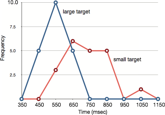
Figure 12. Overlaid frequency polygons.
It is also possible to plot two cumulative frequency distributions in the same graph. This is illustrated in Figure 13 using the same data from the cursor task. The difference in distributions for the two targets is again evident.
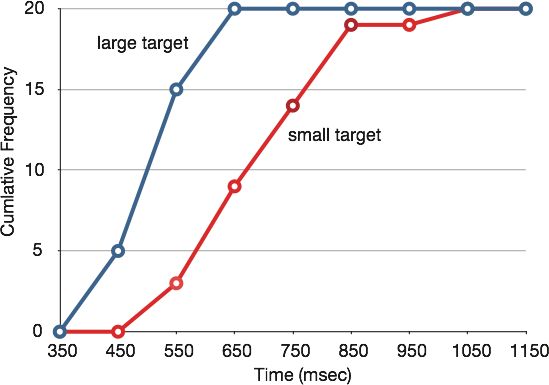
Figure 13. Overlaid cumulative frequency polygons.
Box Plots
We have already discussed techniques for visually representing data (see histograms and frequency polygons). In this section, we present another important graph, called a box plot. Box plots (often called a box-and-whisker plot) are useful for identifying outliers (extreme scores) and for comparing distributions. We will explain box plots with the help of data from an in-class experiment. Students in Introductory Statistics were presented with a page containing 30 colored rectangles. Their task was to name the colors as quickly as possible. Their times (in seconds) were recorded. We’ll compare the scores for the 16 men and 31 women who participated in the experiment by making separate box plots for each group. Such a display is said to involve parallel box plots.
There are several steps in constructing a box plot. The first relies on the 25th, 50th, and 75th percentiles in the distribution of scores. Figure 14 shows how these three statistics are used. For each group we draw a box extending from the 25th percentile to the 75th percentile. The 50th percentile is drawn inside the box.
Therefore, the bottom of each box is the 25th percentile, the top is the 75th percentile, and the line in the middle is the 50th percentile. The data for the women in our sample are shown in Table 6.
|
14, 15, 16, 16, 17, 17, 17, 17, 17, 18, 18, 18, 18, 18, 18, 19, 19, 19, 20, 20, 20, 20, 20, 20, 21, 21, 22, 23, 24, 24, 29 |
Table 6. Women’s times.
Percentiles are determined by dividing data into quarters or quartiles. The 25th percentile is the data point that divides the bottom 25% of the data from the top 75% of the data. The 50th percentile is the data point that divides the bottom 50% from the top 50%. The 75th percentile is the data point that divides the bottom 75% from the top 25%. So, for the women’s scores, with 31 women participating, the 16th score in order would divide the top half from the bottom half. Thus, the 50th percentile is 19. Following the same logic, for these data, the 25th percentile is 17 and the 75th percentile is 20. For the men (whose data are not shown), the 25th percentile is 19, the 50th percentile is 22.5, and the 75th percentile is 25.5.
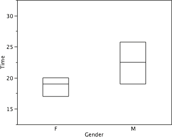
Figure 14. The first step in creating box plots is to identify appropriate quartiles.
Continuing with the box plots, we put “whiskers” above and below each box to give additional information about the spread of data. Whiskers are lines extending from the box plot that represent the majority of bottom and top 25% of your distribution. Whiskers are drawn from the 25th percentile to minimum adjacent value and 75th percentile to the maximum adjacent value (14 and 24, respectively, for the women’s data), as shown in Figure 15.
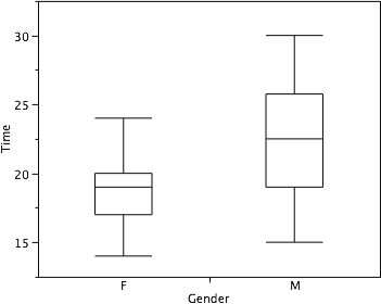
Figure 15. The box plots with the whiskers drawn.
Although whiskers may not cover all data points, we still wish to represent data outside whiskers in our box plots. This is achieved by adding additional marks beyond the whiskers. Specifically, outside (or non-adjacent) values are indicated by small “o’s” and outlier (or extreme) values are indicated by asterisks (*). In our data, there are no far-out or extreme values and just one outside value. This outside value of 29 is for the women and is shown in Figure 16.
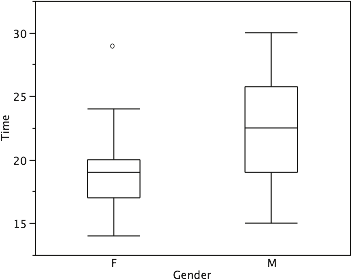
Figure 16. The box plots with the outside value shown.
There is one more mark to include in box plots (although sometimes it is omitted). We indicate the mean (average) score for a group by inserting a plus sign. A mean is one type of central tendency we will learn about in the next chapter. Figure 17 shows the result of adding means to our box plots.
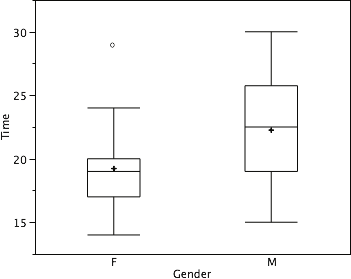
Figure 17. The completed box plots.
Figure 17 provides a revealing summary of the data. Because half the scores in a distribution are between the 25th and 75th percentiles, we see that half the women’s times are between 17 and 20 seconds whereas half the men’s times are between 19 and 25.5 seconds. We also see that women generally named the colors faster than the men did, although one woman was slower than almost all of the men.
The Shape of Distribution
Finally, it is useful to present discussion on how we describe the shapes of distributions, which we will revisit in the next chapter to learn how different shapes affect our numerical descriptors of data and distributions.
The primary characteristic we are concerned about when assessing the shape of a distribution is whether the distribution is symmetrical or skewed. A symmetrical distribution, as the name suggests, can be cut down the center to form 2 mirror images. Although in practice we will never get a perfectly symmetrical distribution, we would like our data to be as close to symmetrical as possible for reasons we delve into in Chapter 4. Many types of distributions are symmetrical, but by far the most common and pertinent distribution at this point is the normal distribution, shown in Figure 18. Notice that although the symmetry is not perfect (for instance, the bar just to the right of the center is taller than the one just to the left), the two sides are roughly the same shape. The normal distribution has a single peak, known as the center, and two tails that extend out equally, forming what is known as a bell shape or bell curve.
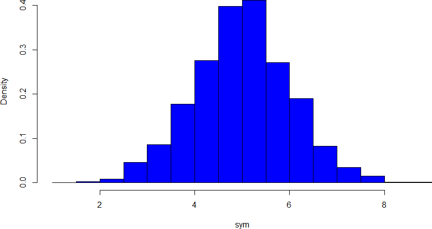
Figure 18. A symmetrical distribution
Symmetrical distributions can also have multiple peaks. Figure 19 shows a bimodal distribution (named for the two peaks) that lie roughly symmetrically on either side of the center point. As we will see in the next chapter, this is not a particularly desirable characteristic of our data, and, worse, this is a relatively difficult characteristic to detect numerically. Thus, it is important to visualize your data before moving ahead with any formal analyses.
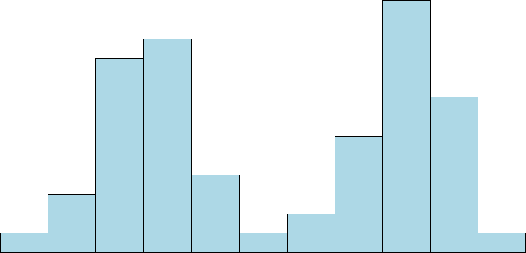
Figure 19. A bimodal distribution
Distributions that are not symmetrical also come in many forms, more than can be described here. The most common asymmetry to be encountered is referred to as skew, in which one of the two tails of the distribution is disproportionately longer than the other. This property can affect the value of the averages we use in our analyses and make them an inaccurate representation of our data, which causes many problems.
Skew can either be positive or negative (also known as right or left, respectively), based on which tail is longer. It is very easy to get the two confused at first; many students want to describe the skew by where the bulk of the data (larger portion of the histogram, known as the body) is placed, but the correct determination is based on which tail is longer. You can think of the tail as an arrow: whichever direction the arrow is pointing is the direction of the skew. Figures 20 and 21 show positive (right) and negative (left) skew, respectively.
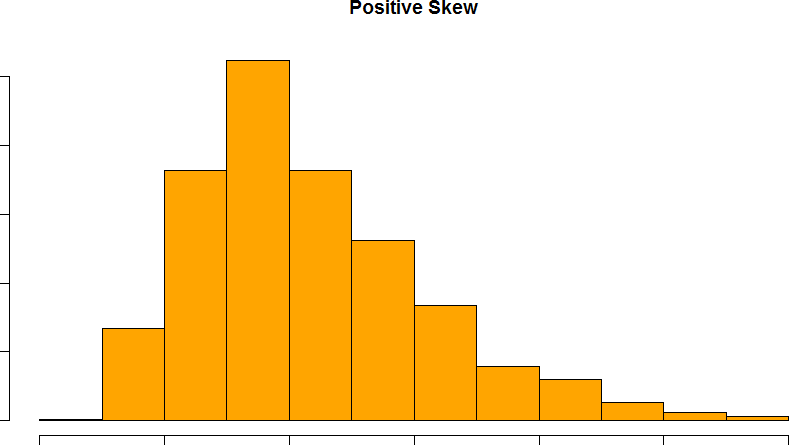
Figure 20. A positively skewed distribution
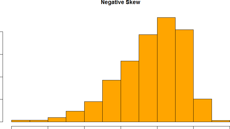
Figure 21. A negatively skewed distribution
Recap
Whether you are using a table or a graph the same two elements of frequency distribution must be present:
- the entire set of categories that make-up the original distribution must be included
- a record of the frequency, or number of individuals in each category within the distribution must be included
Examining our data graphically is useful and there are different choices in graphing depending on what is needed and the type of data you have. The scale of measurement determines the most appropriate graph to use. Bar graphs are used to display qualitative data along a nominal or ordinal scale of measurement. Histograms, frequency polygons, and box-and-whisker plots are most appropriate when using interval or ratio scales of measurement.
Key Takeaway: which graph can go with what levels of measurement?!
| Level of Measurement | Graph |
| Nominal | Pie chart
Bar graph Grouped bar graph |
| Ordinal | Bar graph
Grouped bar graph |
| Interval | Frequency polygon
Line graph Box-and-whiskers plot Histogram |
| Ratio | Frequency polygon
Line graph Box-and-whiskers plot Histogram |
- Figure 1: An image of the solid rocket booster leaking fuel, seconds before the explosion. The small flame visible on the side of the rocket is the site of the O-ring failure. By NASA (Great Images in NASA Description) [Public domain], via Wikimedia Commons ↵
Techniques that organize, summarize, and describe a set of data.
A table or graph that breaks down the number of times or occurrence of a particular category or value of a variable of interest in your data.
Observation or data point that does not fit the pattern of the rest of the data. Sometimes called an extreme value.
How many times a particular category occurs.
A ratio of occurrence for a particular category in a set of data. It is calculated by dividing the frequency of a category by the total number of observations or data points in that dataset.
a graph in which bars of varying height with spaces between them are used to display data for variables defined by qualities or categories.
a graphical depiction of continuous data using bars of varying height, similar to a bar graph but with blocks on the x-axis adjoining or touching one another so as to show their continuous nature. A histogram is appropriate to use when data is measured on an interval or ratio scale.
A group of scores in a grouped frequency distribution. Groups of scores have the same range (e.g., grouped by 10s)
The proportion of the total distribution rather than the absolute frequency. Used for population distributions for which the absolute number of individuals is not known for each category.
a graph depicting a statistical distribution, made up of lines connecting the peaks of adjacent intervals. A line graph connecting the midpoints of the bars of a histogram is a frequency polygon.
a graphical display of the central value, variance, and extreme values in a data set. Used to identify outliers and for comparing distributions. Also known as box-and-whisker plots.
the location of a score in a distribution expressed as the percentage of cases in the data set with scores equal to or below the score in question.
values that divide a list of numbers into quarters. For example, the first (or lower) quartile of a distribution is the data value below which are the lowest 25% of scores, the second quartile is the data value below which are 50% of scores, and the third (or upper) quartile is the data value below which are 75% of scores (or, conversely, above which are 25% of scores).
lines extending from the box plot that represent the majority of bottom and top 25% of your distribution.
a distribution in which the frequency of values above the mean are a mirror image of those below the mean.
