The Vocabulary of Statistical Investigations

Jennifer Ivie; Alicia MacKay

2 The Vocabulary of Statistical Investigations

Learning Outcomes

In this chapter, you will learn how to:

Define the terminology.
Differentiate the different types of research design.
Differentiate the different types of sampling.
Distinguish between different types of variables.
Distinguish between the concepts of reliability and validity.
Use the special notations of statistics

In order to use statistics, we need data to analyze. Data come in an amazingly diverse range of formats, and each type gives us a unique type of information. In virtually any form, data represent the measured value of variables. A variable is simply a characteristic or feature of the thing we are interested in understanding. Let’s imagine we want to conduct a study to measure the stress level of students who are taking Introductory Statistics. We will administer the survey during the first week of the course. One question we will ask is, “How stressed have you been in the last 2 weeks, on a scale of 0 to 10, with 0 being not at all stressed and 10 being as stressed as possible?”

A Variable is a condition or characteristic that can take on different values. In our example, the variable was stress, which can take on any value between 0 and 10. Height is a variable. Social class is a variable. One’s score on a creativity test is a variable. The number of people absent from work on a given day is a variable. In psychology, we are interested in people, so we might get a group of people together and measure their levels of anxiety (a variable) or their physical health (another variable). You get the point. Pretty much anything we can count or measure can be a variable.
- Once we have data on different variables, we can use statistics to understand if and how they are related.

A value is just a number, such as 4, – 81, or 367.12. A value can also be a category (word), such as male or female, or a psychological diagnosis (major depressive disorder, post-traumatic stress disorder, schizophrenia).
- We will learn more about values and types of data a little later in this chapter.

Each person studied has a particular score that is his or her value on the variable. As we’ve said, your score on the stress variable might have a value of 6. Another student’s score might have a value of 8.

We also need to understand the nature of our data: what they represent and where they came from. Here are a few key considerations for using statistics.

Know the basic components of a statistical investigation.
Know the sample. Identify if using a representative sample.
Identify the sample size. Evaluate if using a large enough sample.
Understand and evaluate the study design.
Identify type of data working with.
Understand the statistics to be used.
Evaluate conclusions made from statistical findings.

The basic components to a statistical investigation

Planning the study: Start by asking a testable research question and deciding how to collect data.

Examining the data: What are appropriate ways to examine the data? What graphs are relevant, and what do they reveal? What descriptive statistics can be calculated to summarize relevant aspects of the data, and what do they reveal? What patterns do you see in the data? Are there any individual observations that deviate from the overall pattern, and what do they reveal?

Inferring from the data: What are valid statistical methods for drawing inferences “beyond” the data you collected?

Drawing conclusions: Based on what you learned from your data, what conclusions can you draw? Who do you think these conclusions apply to? Can you draw a cause-and-effect conclusion about your treatment? (Note: we are about to learn more about the study design needed for this)

The numerical analysis (“crunching numbers” on the computer) comprises only a small part of the overall statistical investigation. In this chapter, you will see how we can answer some of these questions and what questions you should be asking about any statistical investigation you read about. In the end, statistics provides us a way to give a very objective “yes” or “no” answer to the question, “is this treatment or intervention effective and, if so, how effective is it?” Nearly all statistical techniques boil down to answering these questions. Statistics is all about helping make correct and reliable decisions in our chosen field of study. But even if you never plan on conducting research or pursuing a career where you have to use statistics, the material in this course will help you in your daily life. In today’s world of instant gratification, information overload, and the 24-hour news cycle, statistics are thrown at us nonstop. Soon, you will be able to determine if the person or group providing these statistics is being honest or manipulating the data to suit their ideas.

Let’s learn a little bit more about what is needed to know to better understand statistics.

Who are your participants? Who is your population?

Research in psychology typically begins with a general question about a specific group (or groups) of individuals or animals. For example, a researcher might want to know how many homeless people live on the streets in a particular city. Or a researcher might want to know how often married people have sex, as reported by partners separately. In the first example, the researcher is interested in the group of homeless people. In the second example, the researcher may study heterosexual couples and compare the group of men with the group of women. In statistics, we call the entire group that a researcher wishes to study a population. As you can well imagine, a population can be quite large; for example, any student enrolled in college. A researcher might be more specific, limiting the population for a study to college students who have successfully completed a statistics course and who live in the United States.

Populations can obviously vary in size from extremely large to very small, depending on how the researcher defines the population. The population being studied should always be identified by the researcher. In addition, the population can include more than people and animals. A population could be corporations, parts produced in a factory, or anything else a researcher wants to study. Because populations tend to be very large it usually is impossible for a researcher to examine every individual in the population of interest. It is typically not feasible to collect data from an entire population. Therefore, researchers typically select a smaller, more manageable group from the population and limit their studies to the individuals in the selected group. A smaller more manageable group, known as a sample, is used to measure populations.

The participants in the research study are the sample, and the larger group the sample represents is the population. When describing data it is necessary to distinguish whether the data come from a population or a sample.

If data describe a sample they are called statistics.
If data describe a population they are called parameters.

If I had given a statistical attitudes survey to the class, the class would be my sample. I might be interested in all students taking a statistics class for the first time, generalizing my findings to all statistics students would be applying information from my sample to a population. While it might be convenient for me to ask my class, does my class best represent all students taking statistics? I would need to carefully consider selecting the best sample for a population or critically think about the limits for generalizing my findings to a population. While our results would be most accurate if we could study the entire population rather than a sample from it, in most research situations this is not practical. Moreover, the goal of research is usually to make generalizations or predictions beyond what resources would allow. Additionally, sampling is an important concept to consider within the big picture of understanding statistics.

Imagine that we wanted to see if statistics anxiety was related to procrastination. We could measure everyone’s levels of statistics anxiety and procrastination and observe how strongly they were related to each other. This would, however, be prohibitively expensive. A more convenient way is to select a number of individuals randomly from the population and find the relationship between their statistics anxiety and procrastination levels. We could then generalize the findings from this sample to the population. We use statistics, more specifically inferential statistics, to help us generalize from a particular sample to the whole population. Understanding the relationship between populations and their samples is the first vital concept to grasp in this course. Remember that the research started with a general question about the population but to answer the question, a researcher studies a sample and then generalizes the results from the sample to the population. The general rule is to get a large enough sample size and have the sample be a good representation of your population.

Representative Sample

Because we are using samples to generalize to the larger population it is important, vital, that the samples look like the population they came from. When the sample closely matches the population from which it was selected we call this a representative sample. An unrepresentative (biased) sample is a subset of the population that does not have the characteristics typical of the target population. One of the simplest ways to ensure a representative sample is through the use of random sampling.

Random Sampling

Usually, the ideal sampling method is called random selection or sampling. The researcher starts with a complete list of the population and randomly selects some of them to study. Random sampling is considered a fair way of selecting a sample from a given population since every member is given equal opportunities of being selected.

Example #1: You have been hired by the National Election Commission to examine how the American people feel about the fairness of the voting procedures in the U.S. Who will you ask?

It is not practical to ask every single American how he or she feels about the fairness of the voting procedures. Instead, we query a relatively small number of Americans, and draw inferences about the entire country from their responses. The Americans actually queried constitute our sample of the larger population of all Americans.

In the case of voting attitudes, we would sample a few thousand Americans drawn from the hundreds of millions that make up the country. In choosing a sample, it is therefore crucial that it not over-represent one kind of citizen at the expense of others. For example, something would be wrong with our sample if it happened to be made up entirely of Florida residents. If the sample held only Floridians, it could not be used to infer the attitudes of other Americans. The same problem would arise if the sample were comprised only of Republicans. Inferences from statistics are based on the assumption that sampling is representative of the population. If the sample is not representative, then the possibility of sampling bias occurs. Sampling bias means that our conclusions apply only to our sample and are not generalizable to the full population.

To solidify your understanding of sampling bias, consider the following example. Try to identify the population and the sample, and then reflect on whether the sample is likely to yield the information desired.

Example #2: A substitute teacher wants to know how students in the class did on their last test. The teacher asks the 10 students sitting in the front row to state their latest test score. He concludes from their report that the class did extremely well. What is the sample? What is the population? Can you identify any problems with choosing the sample in the way that the teacher did?

In Example #2, the population consists of all students in the class. The sample is made up of just the 10 students sitting in the front row. The sample is not likely to be representative of the population. Those who sit in the front row tend to be more interested in the class and tend to perform higher on tests. Hence, the sample may perform at a higher level than the population.

Simple Random Sampling

Researchers adopt a variety of random sampling strategies. The most straightforward is simple random sampling. Such sampling requires every member of the population to have an equal chance of being selected into the sample. In addition, the selection of one member must be independent of the selection of every other member. That is, picking one member from the population must not increase or decrease the probability of picking any other member (relative to the others). In this sense, we can say that simple random sampling chooses a sample by pure chance. To check your understanding of simple random sampling, consider the following example.

What is the population? What is the sample? Was the sample picked by simple random sampling? Is it biased?

Example #3: A research scientist is interested in studying the experiences of twins raised together versus those raised apart. She obtains a list of twins from the National Twin Registry, and selects two subsets of individuals for her study. First, she chooses all those in the registry whose last name begins with Z. Then she turns to all those whose last name begins with B. Because there are so many names that start with B, however, our researcher decides to incorporate only every other name into her sample. Finally, she mails out a survey and compares characteristics of twins raised apart versus together.

In Example #3, the population consists of all twins recorded in the National Twin Registry. It is important that the researcher only make statistical generalizations to the twins on this list, not to all twins in the nation or world. That is, the National Twin Registry may not be representative of all twins. You may have guess this is not a simple random sample. Choosing only twins whose last names begin with Z and B does not give every individual an equal chance of being selected into the sample.

Sample size matters

Recall that the definition of a random sample is a sample in which every member of the population has an equal chance of being selected. This means that the sampling procedure rather than the results of the procedure define what it means for a sample to be random. Random samples, especially if the sample size is small, are not necessarily representative of the entire population. Only a large sample size makes it likely that our sample is close to representative of the population. For this reason, inferential statistics take into account the sample size when generalizing results from samples to populations. In later chapters, you’ll see what kinds of mathematical techniques ensure this sensitivity to sample size.

More complex sampling

Sometimes it is not feasible to build a sample using simple random sampling. For this reason, other kinds of sampling techniques have been devised. We now discuss two of them.

Stratified Sampling

Since simple random sampling often does not ensure a representative sample, a sampling method called stratified random sampling is sometimes used to make the sample more representative of the population. This method can be used if the population has a number of distinct “strata” or groups. In stratified sampling, you first identify members of your sample who belong to each group. Then you randomly sample from each of those subgroups in such a way that the sizes of the subgroups in the sample are proportional to their sizes in the population.

Let’s take an example: Suppose you were interested in views of capital punishment at an urban university. You have the time and resources to interview 200 students. The student body is diverse with respect to age; many older people work during the day and enroll in night courses (average age is 39), while younger students generally enroll in day classes (average age of 19). It is possible that night students have different views about capital punishment than day students. If 70% of the students were day students, it makes sense to ensure that 70% of the sample consisted of day students. Thus, your sample of 200 students would consist of 140 day students and 60 night students. The proportion of day students in the sample and in the population (the entire university) would be the same. Inferences to the entire population of students at the university would therefore be more accurate.

Convenience Sampling

Unfortunately, it is often impractical or impossible to study a truly random sample. Much of the time, in fact, studies are conducted with whoever is willing or available to be a research participant – this is commonly referred to as convenience sampling.

Psychologists have been guilty of largely recruiting samples of convenience from the thin slice of humanity—students—found at universities and colleges (Sears, 1986). This presents a problem when trying to assess the social mechanics of the public at large. Aside from being an overrepresentation of young, middle-class Caucasians, college students may also be more compliant and more susceptible to attitude change, have less stable personality traits and interpersonal relationships, and possess stronger cognitive skills than samples reflecting a wide range of age and experience (Peterson & Merunka, 2014; Visser, Krosnick, & Lavrakas, 2000). Put simply, these traditional samples (college students) may not be sufficiently representative of the broader population. Furthermore, considering that 96% of participants in psychology studies come from western, educated, industrialized, rich, and democratic countries (so-called WEIRD cultures; Henrich, Heine, & Norenzayan, 2010), and that the majority of these are also psychology students, the question of non-representativeness becomes even more serious. Of course, when studying a basic cognitive process (like working memory capacity) or an aspect of social behavior that appears to be fairly universal (e.g., even cockroaches exhibit social facilitation), a non-representative sample may not be a big deal.

Type of Research Designs

Research studies come in many forms, and, just like with the different types of data we have, different types of studies tell us different things. The choice of research design is determined by the research question. Though a complete understanding of different research designs is the subject for at least one full class, if not more, a basic understanding of the principles is useful here. There are three types of research designs we will discuss: non-experimental, quasi-experimental, and experimental.

Non-Experimental Designs

Non-experimental research (often called correlational research) involves observing things as they occur naturally and recording our observations as data in order to find a relationship between variables.

Consider this example: A data scientist wants to know if there is a relationship between how conscientious a person is and whether that person is a good employee. She hopes to use this information to predict the job performance of future employees by measuring their personality when they are still job applicants. She randomly samples volunteer employees from several different companies, measuring their conscientiousness and having their bosses rate their performance on the job. She analyzes this data to find a relationship. Conscientiousness is a person-based variable that a researcher must gather data from employees as they are in order to find a relation between her variables.

Though this type of research design cannot establish causality, it can still be quite useful. If the relationship between conscientiousness and job performance is consistent, then it doesn’t necessarily matter if conscientiousness causes good performance or if they are both caused by something else – she can still measure conscientiousness to predict future performance. Additionally, these studies have the benefit of reflecting reality as it actually exists since we as researchers do not change anything.

Experimental Designs

If we want to know if a change in one variable causes a change in another variable, we must use a true experiment. A true experiment is an experimental design with random assignment. In an experimental design a researcher assigns or manipulates which groups the participants will be in. Further, each participant is randomly assigned to a group. If there is no random assignment, the experiment can not have cause-effect conclusions.

Types of Variables in an Experiment

When conducting research, researchers often manipulate variables. For example, a researcher might compare the effectiveness of four types of antidepressants. In this case, the variable is “type of antidepressant.” When a variable is manipulated by an experimenter, it is called an independent variable. The researcher seeks to determine the effect of the independent variable on relief from depression. In this example, relief from depression is called a dependent variable. In general, the independent variable is manipulated by the researcher and its effects on the dependent variable are measured.

To understand what this means, let’s look at an example: A clinical researcher wants to know if a newly developed drug is effective in treating the flu. Working with collaborators at several local hospitals, she randomly samples 40 flu patients and randomly assigns each one to one of two conditions: Group A receives the new drug and Group B receives a placebo. She measures the symptoms of all participants after 1 week to see if there is a difference in symptoms between the groups.

In the example, the independent variable is the drug treatment; we manipulate it into 2 levels: new drug or placebo. Each person, after being randomly sampled to be in the research, was then randomly assigned to one of the 2 groups. That is, random sampling and random assignment are not the same thing and cannot be used interchangeably. For research to be a true experiment, random assignment must be used. The dependent variable in the example is flu symptoms. Barring any other intervention, we would assume that people in both groups, on average, get better at roughly the same rate. Because there are no systematic differences between the 2 groups, if the researcher does find that Group A has a decrease in symptoms, she can confidently attribute it to the effectiveness of the new drug.

Can you identify the independent and dependent variables?

Example #1: Can blueberries slow down aging? A study indicates that antioxidants found in blueberries may slow down the process of aging. In this study, 19-month- old rats (equivalent to 60-year-old humans) were fed either their standard diet or a diet supplemented by either blueberry, strawberry, or spinach powder (randomly assigned). After eight weeks, the rats were given memory and motor skills tests. Although all supplemented rats showed improvement, those supplemented with blueberry powder showed the most notable improvement.

What is the independent variable? (dietary supplement: none, blueberry, strawberry, and spinach)
What are the dependent variables? (memory test and motor skills test)

Example #2: Does beta-carotene protect against cancer? Beta-carotene supplements have been thought to protect against cancer. However, a study published in the Journal of the National Cancer Institute suggests this is false. The study was conducted with 39,000 women aged 45 and up. These women were randomly assigned to receive a beta-carotene supplement or a placebo, and their health was studied over their lifetime. Cancer rates for women taking the beta-carotene supplement did not differ systematically from the cancer rates of those women taking the placebo.

What is the independent variable? (supplements: beta-carotene or placebo)
What is the dependent variable? (occurrence of cancer)

Levels of an Independent Variable

In order to establish that one variable must cause a change in another variable, a researcher will likely use two or more groups or levels.

Experimental (treatment) group(s) is the group who is exposed to the treatment. You can have more than one treatment group (as in Blueberry supplement example above).

Control group is the group who is not exposed to the treatment; the control group serves as the comparison group.

If an experiment compares an experimental group with a control group, then the independent variable (type of treatment) has two levels: experimental and control. Further, if an experiment were comparing five types of diets, then the independent variable (type of diet) would have 5 levels. In general, the number of levels of an independent variable is the number of experimental group and control group combined.

Quasi-Experimental Designs

Quasi-experimental research involves getting as close as possible to the conditions of a true experiment when we cannot meet all requirements. Specifically, in a quasi-experimental design a researcher is looking for group differences but does not or cannot randomly assign people to groups. There are several reasons this might be used. First, it may be unethical to randomly assign participants to a particular experimental group. For example, assigning participants to smoke cigarettes if they are non-smokers. Alternatively, it may be impossible to randomly assign people to groups (e.g., gender or age groups).

Or consider another example: A professor wants to test out a new teaching method to see if it improves student learning. Because he is teaching two sections of the same course, he decides to teach one section the traditional way and the other section using the new method. At the end of the semester, he compares the grades on the final for each class to see if there is a difference.

In this example, the professor has manipulated his teaching method, which is the independent variable, hoping to find a difference in student performance, the dependent variable. However, because students enroll in courses, he cannot randomly assign the students to a particular group, thus precluding using a true experiment to answer his research question. Because of this, we cannot know for sure that there are no systematic differences between the classes other than teaching style and therefore cannot determine causality.

Extraneous and Confounding Variables

Sometimes in a research study things happen that make it difficult for a researcher to determine whether the independent variable caused the change in the dependent variable. These have special names.

An extraneous variable is something that occurs in the environment or happens to the participants that could unintentionally influence the outcome of the study.

A confounding variable is a type of extraneous variable that will influence the outcome of the study. And so, researchers do their best to control these variables.

Working with data

What are data?

The first important point about data is that data are – meaning that the word “data” is plural (though some people disagree with us on this). According to the American Psychological Association, data are observations or measurements, usually quantified and obtained in the course of research (2022).

Operationalizing Variables

We need to have specifically defined how we are measuring our construct or our variable. The act of defining how to measure a variable is to create an operational definition. Some variables are easier to define, like height or weight. I can measure height in inches or weight in pounds. Some other variables can be more abstract, like happiness or love. How would I measure happiness? Would I simply ask are you happy (yes or no)? Would I use a questionnaire for a self-report measure? Would I rate individuals from observing them for happiness? Would I ask their partner, teacher, parent, best friend about the person’s happiness? Researchers’ decisions on how to measure data are an important factor and helps to determine what kind of data are being used.

Image Source

How would you measure happiness in a research study?

Qualitative and Quantitative Variables

Data are composed of variables, where a variable reflects a unique measurement or quantity. An important distinction between variables is between qualitative variables and quantitative variables. Qualitative variables are those that express a qualitative attribute such as hair color, eye color, religion, favorite movie, gender, and so on. Qualitative means that they describe a quality rather than a numeric quantity. Qualitative variables are sometimes referred to as categorical variables. For qualitative variables, response options are usually limited or fixed to a set of possible values.

More commonly in statistics we will work with quantitative data, meaning data that are numerical. Quantitative variables are those variables that are measured in terms of numbers. Some examples of quantitative variables are height, weight, and shoe size.

All studies can involve qualitative and quantitative data. In the study on the effect of diet discussed previously, the independent variable was type of supplement: none, strawberry, blueberry, and spinach. The variable “type of supplement” is a qualitative variable; there is nothing quantitative about it. In contrast, the dependent variable “memory test” is a quantitative variable since memory performance was measured on a quantitative scale (number correct).

Discrete and Continuous Variables

Variables such as number of children in a household are called discrete variables because the possible scores are separate categories on the scale. For example, a household could have three children or six children, but not 4.53 children. Other variables such as “time to respond to a question” are continuous variables since the scale is continuous and not made up of discrete steps. The response time could be 1.64 seconds, or it could be 1.64237123922121 seconds. Of course, the practicalities of measurement preclude most measured variables from being truly continuous.

Levels of Measurement

Numbers mean different things in different situations. Consider these questions about a race that you just finished:

What number were you wearing in the race?
What place did you finish in?
What running shoe size did you wear?
How many minutes did it take you to finish the race?

What if your answer to all four questions was 8?

The four variables (identification number, finish place, shoe size, and time) are quite different. Because of these different variables, the way we interpret 8 is unique for each variable. To illustrate the difference, consider your friend who also ran the race. Their answers to the same three questions were 10, 10, 10, and 10. If we take the first question by itself and know that you had a score of 8, and your friend had a score of 10, what can we conclude? We can conclude that your race identification number is different from your friend’s number. That is all we can conclude. On the second question, with scores of 8 and 10, what can we conclude regarding the place you and your friend finished in the race? We can state that you were faster than your friend in the race and, of course, that your finishing places are different. Comparing the 8 and 10 on the third question, what can we conclude? We could state that your friend’s shoe size went up two intervals (depending on gender). Comparing the 8 and 10 on the fourth question, what can we conclude? We could state that you ran the race 25% faster than your friend, you ran the race faster than your friend and that your time was different than your friend’s time.

The point of this discussion is to demonstrate the types of descriptive and inferential statistics we can use depend on the type of variable measured. Remember, a variable is defined as a characteristic we can measure that can assume more than one value.

For statistical analysis, exactly how the measurement is carried out depends on the type of variable involved in the analysis. Different types are measured differently. There are four different levels of measurement (also called “scales of measurement”.) The four scales of measurement include: nominal, ordinal, interval, and ratio.

Nominal scales

When measuring using a nominal scale, one simply names or categorizes responses. Gender, handedness, favorite color, and religion are examples of variables measured on a nominal scale. The essential point about nominal scales is that they do not imply any ordering among the responses. Responses are merely categorized. For example, when classifying people according to their favorite color, there is no sense in which green is placed “ahead of” blue. In our number example above, the number you were wearing in the race would be measured on a nominal scale of measurement. Nominal scales embody the lowest level of measurement.

Ordinal scales

A researcher wishing to measure consumers’ satisfaction with their microwave ovens might ask them to specify their feelings as either “very dissatisfied,” “somewhat dissatisfied,” “somewhat satisfied,” or “very satisfied.” The items in this scale are ordered, ranging from least to most satisfied. This is what distinguishes ordinal from nominal scales. Unlike nominal scales, ordinal scales allow researchers to make comparisons between categories of the variable. However, the distance between categories is not measured. In the race example above, the place you finished in would be measured on an ordinal scale.

(Equal) Interval scales

Interval scales is a scale of measurement where the difference between two consecutive values is equal regardless of the value selected. For the race example above, your shoe size would be measured on an interval scale. The distance between each shoe size is the same (the distance from a size 4 to 6 is the same as the distance from a size 8 to 10). Another example of an interval scale of measurement is the time of day; 3 pm is one hour later than 2 pm just like 7am is one hour later than 6am).

Ratio scales (Absolute zero)

The ratio scale of measurement is the most informative scale. It is an interval scale with the additional property that its zero position indicates the absence of the quantity being measured. You can think of a ratio scale as the three earlier scales rolled up in one. Like a nominal scale, it provides a name or category for each object (the numbers serve as labels). Like an ordinal scale, the objects are ordered (in terms of the ordering of the numbers). Like an interval scale, the same difference at two places on the scale has the same meaning. And in addition, the same ratio at two places on the scale also carries the same meaning.

In the race example above, the time you took to finish the race is measured on a ratio scale. Time is measured on a ratio scale because you can express it in terms of a ratio; you finished in 8/10 time or 25% faster than your friend. Another example of a ratio scale is the amount of money you have in your pocket right now (25 cents, 55 cents, etc.). Money is measured on a ratio scale because, in addition to having the properties of an interval scale, it has a true zero point: if you have zero money, this implies the absence of money. Since money has a true zero point, it makes sense to say that someone with 50 cents has twice as much money as someone with 25 cents (or that Bill Gates has a million times more money than you do).

Digging deeper: What about the number value? It is important to know what number values mean. Is the number meaningful or it is a category? This section briefly reviews how numbers can be categorized according to meaning.

Binary numbers. The simplest are binary numbers – that is, zero or one. We will often use binary numbers to represent whether something is true or false, or present or absent. For example, I might ask 10 people if they have ever experienced a migraine headache, recording their answers as “Yes” or “No”. It’s often useful to instead use logical values, which take the value of either TRUE or FALSE. This can be especially useful for programming languages to analyze data, since these languages already understand the concepts of TRUE and FALSE. In fact, most programming languages treat truth values and binary numbers equivalently. The number 1 is equal to the logical value TRUE, and the number zero is equal to the logical value FALSE.

Integers. Integers are whole numbers with no fractional or decimal part. We most commonly encounter integers when we count things, but they also often occur in psychological measurement. For example, in my introductory survey I administer a set of questions about attitudes towards statistics (such as “Statistics seems very mysterious to me.”), on which the students respond with a number between 1 (“Disagree strongly”) and 7 (“Agree strongly”). Integers are discontinuous.

Real numbers. Most commonly in statistics we work with real numbers, which have a fractional/decimal part. For example, we might measure someone’s weight, which can be measured to an arbitrary level of precision, from kilograms down to micrograms. Real numbers can be discontinuous or continuous.

Consequences of level of measurement

Why are we so interested in the type of scale that measures a variable? The crux of the matter is the relationship between the variable’s level of measurement and the statistics that can be meaningfully computed with that variable. For example, consider a hypothetical study in which 5 children are asked to choose their favorite color from blue, red, yellow, green, and purple. The researcher codes the results as follows:

Color	Code
Blue	1
Red	2
Yellow	3
Green	4
Purple	5

This means that if a child said her favorite color was “Red,” then the choice was coded as “2,” if the child said her favorite color was “Purple,” then the response was coded as 5, and so forth. Consider the following hypothetical data:

Subject	Color	Code
1	Blue	1
2	Blue	1
3	Green	4
4	Green	4
5	Purple	5

Each code is a number, so nothing prevents us from computing the average code assigned to the children. The average happens to be 3, but you can see that it would be senseless to conclude that the average favorite color is yellow (the color with a code of 3). Such nonsense arises because favorite color is a nominal scale, and taking the average of its numerical labels is like counting the number of letters in the name of a snake to see how long the animal is.

What makes a good measurement?

In many fields such as psychology, the thing that we are measuring is not a physical feature, but instead is an unobservable theoretical concept, which we usually refer to as a construct. For example, let’s say that we want to test how well you understand the distinction between the different types of numbers described above. We could give you a pop quiz that would ask you several questions about these concepts and count how many you got correct. If we were to write the test in a confusing way or use language that you don’t understand, then the test might suggest you don’t understand the concepts when really you do. On the other hand, if we give a multiple-choice test with very obvious wrong answers, then you might be able to perform well on the test even if you don’t actually understand the material. This test might or might not be a good measurement of the construct of your actual knowledge. When we think about what makes a good measurement, we usually distinguish two different aspects of a good measurement: it should be reliable, and it should be valid.

Reliability

Reliability refers to the consistency of our measurements. One common form of reliability, known as test-retest reliability, measures how well the measurements agree if the same measurement is performed twice. For example, if you took the ACT today and again in 6 months, unless you increase your study time, your scores should be similar.

Another way to assess reliability comes in cases where the data include subjective judgments. For example, let’s say that a researcher wants to determine whether a treatment changes how well an autistic child interacts with other children, which is measured by having experts watch the child and rate their interactions with the other children. In this case we would like to make sure that the answers don’t depend on the individual rater — that is, we would like for there to be high inter-rater reliability. This can be assessed by having more than one rater perform the rating, and then comparing their ratings to make sure that they agree well with one another.

Validity

Reliability is important, but on its own it’s not enough. After all, I could create a perfectly reliable measurement on a personality test by re-coding every answer using the same number, regardless of how the person actually answers. We want our measurements to also be valid — that is, we want to make sure that we are actually measuring the construct that we think we are measuring (Figure 1). There are many different types of validity that are commonly discussed; we will focus on three of them.

Face validity. Does the measurement make sense? If I were to tell you that I was going to measure a person’s blood pressure by looking at the color of their tongue, you would probably think that this was not a valid measure . On the other hand, using a blood pressure cuff would have face validity. This is usually a first reality check before we dive into more complicated aspects of validity.

Construct validity. Is the measurement related to other measurements in an appropriate way? This is often subdivided into two aspects. Convergent validity means that the measurement should be closely related to other measures that are thought to reflect the same construct. Let’s say that we are interested in measuring how extroverted a person is using either a questionnaire or an interview. Convergent validity would be demonstrated if both of these different measurements are closely related to one another. On the other hand, measurements thought to reflect different constructs should be unrelated, known as divergent validity. If a theory of personality says that extraversion and conscientiousness are two distinct constructs, then we should also see that our measurements of extraversion are unrelated to measurements of conscientiousness.

Predictive validity. If our measurements are truly valid, then they should also be predictive of other outcomes. For example, let’s say that we think that the psychological trait of sensation seeking (the desire for new experiences) is related to risk taking in the real world. To test for predictive validity of a measurement of sensation seeking, we would test how well scores on the test predict scores on a different survey that measures real-world risk taking.

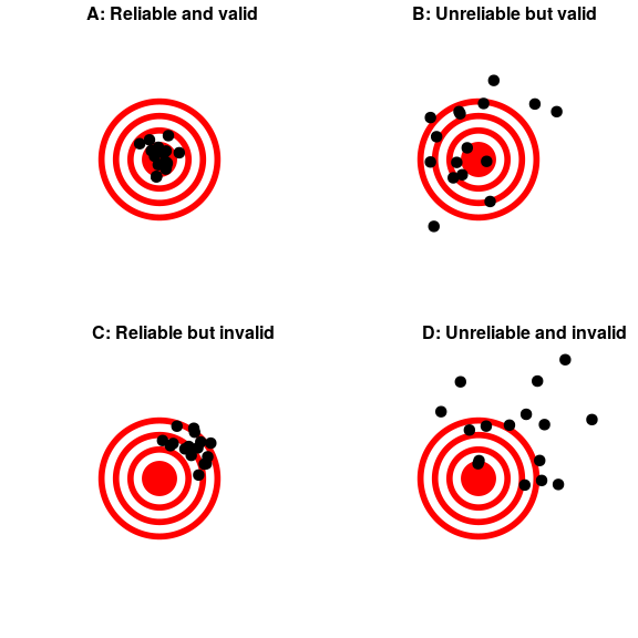
A figure demonstrating the distinction between reliability and validity, using shots at a bullseye. Reliability refers to the consistency of location of shots, and validity refers to the accuracy of the shots with respect to the center of the bullseye.

Figure 1. A figure demonstrating the distinction between reliability and validity, using shots at a bullseye. Reliability refers to the consistency of location of shots, and validity refers to the accuracy of the shots with respect to the center of the bullseye.

Critical Evaluation of Statistical Results

We need to critically evaluate the statistical studies we read about before accepting the results of the studies. Common problems to be aware of include:

Problems with samples: A sample must be representative of the population. A sample that is not representative of the population is biased. Biased samples that are not representative of the population give results that are inaccurate and not valid.
Self-selected samples: Responses only by people who choose to respond, such as call-in surveys, are often unreliable.
Sample size issues: Samples that are too small may be unreliable. Larger samples are better, if possible. In some situations, having small samples is unavoidable and can still be used to draw conclusions.
Undue influence: Collecting data or asking questions in a way that influences the response can make the results invalid.
Non-response or refusal of a participant to participate: The collected responses may not be representative of the population. Often, people with strong positive or negative opinions may answer surveys, which can affect the results.
Causality: A relationship between two variables does not mean that one causes the other to occur. They may be related (correlated) because of their relationship through a different variable.
Self-funded or self-interest studies: A study performed by a person or organization in order to support their claim cannot be impartial. Read the study carefully to evaluate the work. Do not automatically assume that the study is good, but do not automatically assume the study is bad either. Evaluate it on its merits and the work done.
Misleading use of data: Improperly displayed graphs, incomplete data, or lack of context can lead to the misuse/misinterpretation of data.
Confounding: When there are confounding variables it makes it difficult or impossible to draw valid conclusions about the effect of each factor.

Types of Statistical Analyses

Now that we understand the nature of our data, let’s turn to the types of statistics we can use to interpret them. As mentioned at the end of chapter 1, there are two types of statistics: descriptive and inferential.

Descriptive Statistics

Descriptive statistics are numbers that are used to organize, summarize, and describe data. If we are analyzing birth certificates, for example, a descriptive statistic might be the percentage of certificates issued in New York State, or the average age of the mother. Any other number we choose to compute also counts as a descriptive statistic for the data from which the statistic is computed. Several descriptive statistics are often used at one time to give a full picture of the data.

Descriptive statistics are just descriptive. They do not involve generalizing beyond the sample. Generalizing from our data to another set of cases is the business of inferential statistics, which you’ll be studying in another section. The remaining chapters of this unit will cover descriptive statistics.

Inferential Statistics

Descriptive statistics are wonderful at telling us what our data look like. However, what we often want to understand is how our data behave. What variables are related to other variables? Under what conditions will the value of a variable change? Are two groups different from each other, and if so, are people within each group different or similar? These are the questions answered by inferential statistics, and inferential statistics are how we generalize from our sample back up to our population.

There are many types of inferential statistics, each allowing us insight into a different behavior of the data we collect. This course will only touch on a small subset (or a sample) of them, but the principles we learn along the way will make it easier to learn new tests, as most inferential statistics follow the same structure and format.

Mathematical Notation

As noted above, statistics is not math. It does, however, use math as a tool. Many statistical formulas involve summing numbers. Fortunately there is a convenient notation for expressing summation. This section covers the basics of this summation notation.

Let’s say we have a variable X that represents the weights (in grams) of 4 grapes:

Grape	X
1	4.6
2	5.1
3	4.9
4	4.4

[latex]\displaystyle\sum_{i=1}^{4} X_i[/latex]

We label Grape 1’s weight X₁, Grape 2’s weight X₂, etc. The following formula means to sum up the weights of the four grapes.

The Greek letter Σ “sigma” indicates summation. The “i = 1” at the bottom indicates that the summation is to start with X₁ and the 4 at the top indicates that the summation will end with X₄. The “X_i” indicates that X is the variable to be summed as i goes from 1 to 4. Therefore,

[latex]\displaystyle\sum_{i=1}^{4} X_i = X_1 + X_2 + X_3 + X_4 = 4.6 + 5.1 + 4.9 + 4.4 = 19[/latex]

The symbol

[latex]\displaystyle\sum_{i=1}^{3} X_i[/latex]

indicates that only the first 3 scores are to be summed. The index variable i goes from 1 to 3.

When all the scores of a variable (such as X) are to be summed, it is often convenient to use the following abbreviated notation:

[latex]\displaystyle\sum X[/latex]

Thus, when no values of i are shown, it means to sum all the values of X.

Many formulas involve squaring numbers before they are summed. This is indicated as

[latex]\displaystyle\sum X^2 = 4.6^2 + 5.1^2 + 4.9^2 + 4.4^2[/latex]

= 21.16 + 26.01 + 24.01 + 19.36 = 90.54

Notice that:

[latex]\displaystyle(\sum X)^2\neq \displaystyle\sum X^2[/latex]

because the expression on the left means to sum up all the values of X and then square the sum (19² = 361), whereas the expression on the right means to square the numbers and then sum the squares (90.54, as shown).

Some formulas involve the sum of cross products. Below are the data for variables X and Y. The cross products (XY) are shown in the third column. The sum of the cross products is 3 + 4 + 21 = 28.

X	Y	*XY**
1	3	3
2	2	4
3	7	21

In summation notation, this is written as:

[latex]\displaystyle\sum XY = 28[/latex]

Three key concepts for statistical formulas:

Perform summation in the correct order following the order of operations (PEMDAS).
Typically we will use a set of scores for the mathematical operations/formulas used in statistics.
Each operation, except for summation, creates a new column of numbers. Summation adds up the sum for the column and is typically seen as the last row.

License

Icon for the Creative Commons Attribution-NonCommercial-ShareAlike 4.0 International License

Introduction to Statistics for the Social Sciences Copyright © 2021 by Jennifer Ivie; Alicia MacKay is licensed under a Creative Commons Attribution-NonCommercial-ShareAlike 4.0 International License, except where otherwise noted.