14 Repeated Measures ANOVA
Learning outcomes
In this chapter, you will learn how to:
- Identify when to use a repeated-measures ANOVA
- Conduct a repeated-measures ANOVA hypothesis test
- Evaluate effect size for a repeated-measures ANOVA
- Conduct post hoc tests for a repeated-measures ANOVA
- Identify the advantages of a repeated-measures ANOVA
Repeated Measures Design
In the previous chapter we discussed independent-measures ANOVAs, which are appropriate to use when you have different groups of individuals in each of the conditions. In this chapter we will discuss repeated-measures ANOVAs. A repeated-measure ANOVA is appropriate to use when you have the same group of individuals in all of your conditions. That is, each participant is being measured at least three times. Remember, that to use an ANOVA you need to have at least three conditions.
Partitioning the Sums of Squares
Time to introduce a new name for an idea you learned about last chapter, it’s called partitioning the sums of squares. Sometimes an obscure new name can be helpful for your understanding of what is going on. ANOVAs are all about partitioning the sums of squares. We already did some partitioning in the last chapter. What do we mean by partitioning?
Imagine you had a big empty house with no rooms in it. What would happen if you partitioned the house? What would you be doing? One way to partition the house is to split it up into different rooms. You can do this by adding new walls and making little rooms everywhere. That’s what partitioning means, to split up.
The act of partitioning, or splitting up, is the core idea of ANOVA. To use the house analogy. Our total sums of squares (SS Total) is our big empty house. We want to split it up into little rooms. Before we partitioned SS Total using this formula:
SStotal = SSbetween + SSwithin
Remember, the SSbetween was the variance we could attribute to the means of the different groups, and SSwithin was the leftover variance that we couldn’t explain. SSbetween and SSwithin are the partitions of SStotal, they are the little rooms.
In the between-subjects case above, we got to split SStotal into two parts. This is the first step of the repeated-measures ANOVA; it is identical to the independent-measures ANOVA that was presented in the previous chapter.
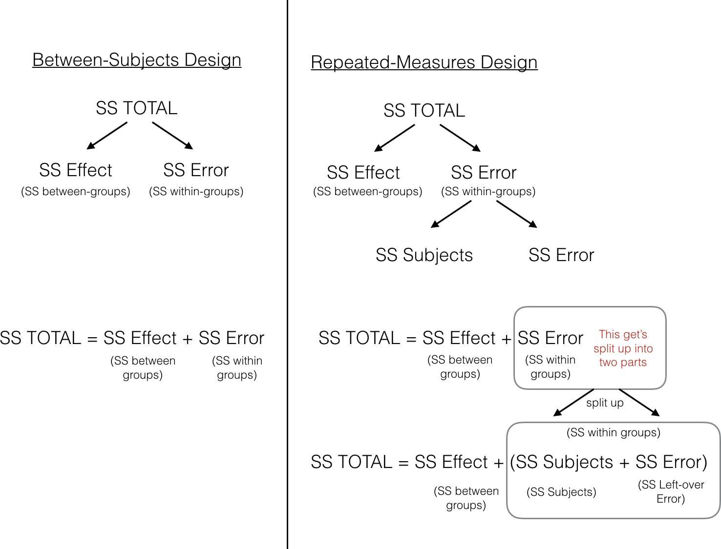
Figure 1. Illustration showing how the total sums of squares are partitioned differently for a between versus repeated-measures design.
The figure lines up the partitioning of the Sums of Squares for both between-subjects and repeated-measures designs. In both designs, SStotal is first split up into two pieces SSbetween treatments (between-groups) and SSwithin. At this point, both ANOVAs are the same. In the repeated measures case we split the SSWithin into two more littler parts, which we call SSbetween subjects (error variation about the subject mean) and SSerror (left-over variation we can't explain). This is the second step in partitioning the Sums of Squares in a repeated-measures ANOVA.
The critical feature of the repeated-measures ANOVA, is that the SSerror that we will later use to compute the MSE in the denominator for the F -value, is smaller in a repeated-measures design, compared to a between subjects design. This is because the SSwithin is split into two parts, SSbetween subjects (error variation about the subject mean) and SSerror (left-over variation we can't explain).
To make this more clear, we made another figure:
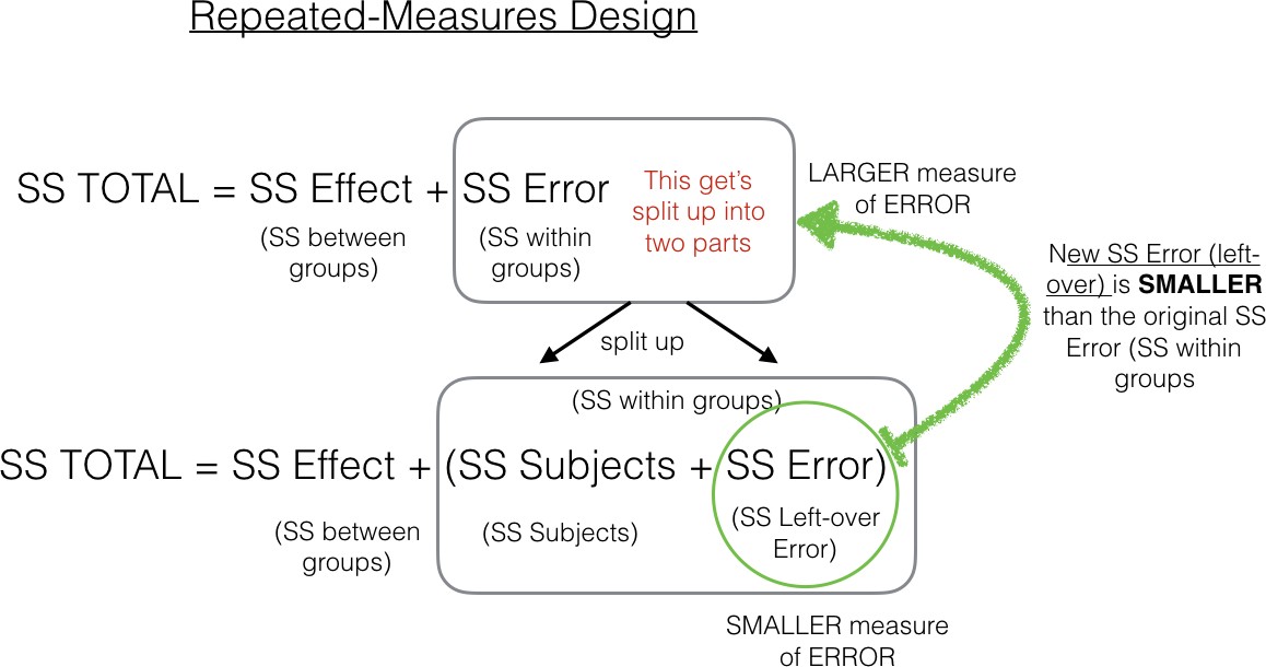
Figure 2. Close-up showing that the Error term is split into two parts in the repeated measures design.
As we point out, the SSerror in the green circle will be a smaller number than the SSwithin. That’s because we are able to subtract out the SSbetween subjects part of the SSwithin. As we will see shortly, this can have the effect of producing larger F-values when using a repeated-measures design compared to a between-subjects design.
Calculating the Repeated-measures ANOVA
Now that you are familiar with the concept of an ANOVA table (remember the table from last chapter where we reported all of the parts to calculate the F -value?), we can take a look at the things we need to find out to make the ANOVA table. The figure below presents an abstract for the repeated-measures ANOVA table. It shows us all the equations we need to calculate to get the F -value for our data. The new rows are covered in the purple equation box below the Source Table.
| Source | SS | df | MS | F |
| Between Treatments | SSbetween treatments | k-1 | [latex]\frac{SS_{between treatments}}{df_{between treatments}}[/latex] | [latex]\frac{MS_{between treatments}}{MS_{error}}[/latex] |
| Within Treatments | SSwithin treatments | N-k | ||
| Between Subjects | SSbetween subjects | n-1 | ||
| Error | SSerror | (N-k)-(n-1) | [latex]\frac{SS_{error}}{df_{error}}[/latex] | |
| Total | SStotal | N-1 |
First, let's review our sums of squares equations from our independent-measures ANOVA that remain in our source table above, the SSbetween treatments, the SSwithin treatments, and the SS total.
SS Total
The total sums of squares, or SStotal measures the total variation in a set of data. All we do is find the difference between each score and the grand mean, then we square the differences and add them all up.
Calculating Total Sums of Squares
Computational Formula
[latex]SS_{total}=\sum(X^2)-\frac{G^2}{N}[/latex]
Where:
X = each individual score within each treatment 1 through k
G = sum of all scores across all treatments 1 through k
N = number of scores across all treatments 1 through k
Definitional Formula
[latex]SS_{total}=\sum(X-M_{grand})^2[/latex]
Where:
X = each individual score within each treatment 1 through k
G = sum of all scores across all treatments 1 through k
Finally, quite simply, the total sum of squares for independent measures ANOVA is just the between groups and the within groups added together.
[latex]SS_{total}=SS_{between treatments}+SS_{within treatments}[/latex]
SS Between Treatments
SStotal gave us a number representing all of the change in our data, how they all are different from the grand mean.
What we want to do next is estimate how much of the total change in the data might be due to the experimental manipulation. For example, if we ran an experiment that causes causes change in the measurement, then the means for each group will be different from other, and the scores in each group will be different from each. As a result, the manipulation forces change onto the numbers, and this will naturally mean that some part of the total variation in the numbers is caused by the manipulation.
The way to isolate the variation due to the manipulation (also called effect) is to look at the means in each group or treatment, and the calculate the difference scores between each group mean and the grand mean, and then the squared deviations to find the sum for SSbetween treatments .
Calculating Sums of Squares for Between Treatments
Computational Formula
[latex]SS_{between treatments}=\displaystyle\sum_{j=1}^{k}\frac{T_j^2}{n_j}-\frac{G^2}{N}[/latex]
Where:
j = “jth” group where j = 1…k to keep track of which treatment mean and sample size we are working with
Tj = sum of scores within treatment j
nj = number of scores within treatment j
G = sum of all scores across all treatments 1 through k
N = number of all scores across all treatments 1 through k
Definitional Formula
[latex]SS_{between treatments}=\displaystyle\sum_{j=1}^{k}\left[\left(M_j-M_{grand}\right)^2*n_j\right][/latex]
Where:
j = “jth” group where j = 1…k to keep track of which treatment mean and sample size we are working with
nj = number of scores within treatment j
Mj = mean of scores within treatment j
Mgrand = mean of scores across all treatments 1 through k
SS within treatments
Great, we made it to SSwithin treatments. We already found SStotal, and SSbetween treatments, so now we can solve for SSwithin treatments just like this:
Calculating Sums of Squares for Within Treatments
[latex]SS_{within treatments}=\displaystyle\sum_{j=1}^{k}SS_j[/latex]
[latex]SS_j=\sum(X_j-M_j)^2[/latex]
Where:
j = “jth” group where j = 1…k to keep track of which treatment mean and sample size we are working with
Xj = a score within treatment j
Mj = mean of scores within treatment j
SS between subjects
Now we are ready to calculate new partition, called SSbetween subjects. This is a measure of the variability between the subjects or participants within each treatment. It takes into account individual differences within each person, hence the person total (P) that is used in the equation below.
Calculating Sums of Squares for Between Subjects
Computational Formula
[latex]SS_{between subjects}=\displaystyle\sum_{j=1}^{n}\frac{P_j^2}{k}-\frac{G^2}{N}[/latex]
Where:
j = “jth” subject where j = 1…n to keep track of which subject total we are working with
Pj = sum of scores within person n
n = number of people within the treatment
G = sum of all scores across all treatments 1 through k
N = number of all scores across all treatments 1 through k
SS Error
Now we can do the last thing. Remember we wanted to split up the SSwithin treatments into two parts, SSbetween subjects and SSerror. Because we have already calculated SSwithin treatments and SSbetween subjects, we can solve for SSerror. It is a simple calculation because it is just what is leftover in our within treatments variability.
Calculating Sums of Squares for Error
[latex]SS_{error}=SS_{within treatments}-SS_{between subjects}[/latex]
We have finished our job of computing the sums of squares that we need in order to do the next steps, which include computing the MSs for the between treatment and the error term. Once we do that, we can find the F-value, which is the ratio of the two MSs.
Before we do that, you may have noticed that we solved for SSerror, rather than directly computing it from the data. In this chapter we are not going to show you the steps for doing this. We are not trying to hide anything from, instead it turns out these steps are related to another important idea in ANOVA. We discuss this idea, which is called an interaction in the next chapter, when we discuss factorial designs (designs with more than one independent variable).
Compute the Mean Squares
Calculating the mean squared error (MS) that we need for the F-value involves the same general steps as last time. We divide each SS by the degrees of freedom for the SS.
The degrees of freedom for SSbetween treatments are the same as before, the number of conditions (k) - 1.
Calculating Degrees of freedom for Between Treatments
[latex]df_{between treatments}=k-1[/latex]
[latex]SS_{error}=SS_{within treatments}-SS_{between subjects}[/latex]
The degrees of freedom for SSerror are the number of subjects (n) - 1 multiplied by the number of conditions (k) - 1. Or, just like above, they are the leftover degrees of freedom when we separate the dfbetween subjects from the dfwithin treatments.
Calculating Degrees of freedom for Error
[latex]df_{error}=(n-1)(k-1)[/latex]
[latex]df_{error}=df_{within treatments}-df_{between subjects}[/latex]
We can then calculate the corresponding mean squared error by dividing the SS by the df. Finally, we calculate our Ftest by dividing our MSbetween treatments by our MSerror this time. Since we were able to account for individual differences by using the same participants across all treatment conditions, we could pull the variability due to between subjects out of the F equation. This left us with pure error in our MSerror value. As you can see in the Source Table repeated below, the MS equations and the Ftest equation are simple ratios of data available in our Source Table.
Compute F in the Source Table
| Source | SS | df | MS | F |
| Between Treatments | SSbetween treatments | k-1 | [latex]\frac{SS_{between treatments}}{df_{between treatments}}[/latex] | [latex]\frac{MS_{between treatments}}{MS_{error}}[/latex] |
| Within Treatments | SSwithin treatments | N-k | ||
| Between Subjects | SSbetween subjects | n-1 | ||
| Error | SSerror | (N-k)-(n-1) | [latex]\frac{SS_{error}}{df_{error}}[/latex] | |
| Total | SStotal | N-1 |
Hypotheses in Repeated-measures ANOVA
The hypotheses for a repeated-measures ANOVA are the same as those for an independent-measures ANOVA - great news, right? That is, the null hypothesis states that there are no mean differences. Remember that we can write this as a sentence or in symbols:
H0: 𝑇ℎ𝑒𝑟𝑒 𝑖𝑠 𝑛𝑜 𝑑𝑖𝑓𝑓𝑒𝑟𝑒𝑛𝑐𝑒 𝑖𝑛 𝑡ℎ𝑒 𝑔𝑟𝑜𝑢𝑝 𝑚𝑒𝑎𝑛𝑠
H0: 𝜇1 = 𝜇2 = 𝜇3
The alternative hypothesis states that there is at least one mean that is different and should be written as follows:
H𝐴: 𝐴𝑡 𝑙𝑒𝑎𝑠𝑡 𝑜𝑛𝑒 𝑚𝑒𝑎𝑛 𝑖𝑠 𝑑𝑖𝑓𝑓𝑒𝑟𝑒𝑛𝑡
EXAMPLE
Let’s look at an example of when we would use a repeated-measures ANOVA. An employer wants to encourage her employees to move more throughout the day so she provided pedometers for a 16-week period. Employees were asked to record their average number of steps per day for weeks 1, 8, and 16. The following table presents the data the employer received for the participating employees (number of steps X 1000).
|
Participant |
Week 1 |
Week 8 |
Week 16 |
P |
| 1 | 7 | 9 | 11 | 27 |
| 2 | 5 | 6 | 7 | 18 |
| 3 | 6 | 6 | 6 | 18 |
| 4 | 2 | 3 | 4 | 9 |
| 5 | 1 | 2 | 3 | 6 |
| 6 | 3 | 4 | 5 | 12 |
| T = 24 | T = 30 | T = 36 | G = 90 | |
| SS = 28 | SS = 32 | SS = 40 | ΣX2 = 562 |
Step 1: State the Hypotheses
Our hypotheses are concerned with the means of groups based on week, so:
H0: 𝑇ℎ𝑒𝑟𝑒 𝑖𝑠 𝑛𝑜 𝑑𝑖𝑓𝑓𝑒𝑟𝑒𝑛𝑐𝑒 in steps based on the week
H0: 𝜇1 = 𝜇2 = 𝜇3
H𝐴: 𝐴𝑡 𝑙𝑒𝑎𝑠𝑡 𝑜𝑛𝑒 𝑚𝑒𝑎𝑛 𝑖𝑠 𝑑𝑖𝑓𝑓𝑒𝑟𝑒𝑛𝑡
Step 2: Find the Critical Values
We will again be using the F distribution table to find our critical values. We will be using two degrees of freedom to find our critical value. These correspond to the numerator and denominator of our test statistic, which for the repeated-measures ANOVA are our Between Groups and Error rows, respectively. The dfbetween treatments is the degrees of freedom value used to calculate the the numerator of our F statistic. Likewise, the dferror is the degrees of freedom value used to calculate the denominator for F.
On most F distribution tables, these are the steps you would use to locate the critical value. For our example, we will use α = .05. The formula for dfbetween treatements is k – 1, and remember that k is the number of groups we are assessing. In this example, k = 3 so our dfbetween treatments = 3-1 = 2. This tells us that we will use the second column, the one labeled 2, to find our critical value. To find the proper row, we simply calculate the dferror, which was (N – k) - (n-1). So we would have (18 - 3) - (6 - 1) = 10. This makes our value for dferror = 10. If we follow the second column down to the row for 10, we find that our critical value is 4.10. We use this critical value the same way as we did before: it is our criterion against which we will compare our obtained test statistic to determine statistical significance. It cuts off the tail or the critical region on the positively skewed F-distribution.
Step 3: Calculate the Test Statistic
Now that we have our hypotheses and the criterion we will use to test them, we can calculate our test statistic. To do this, we will fill in the ANOVA source table. When we do so, we will work our way from left to right, filling in each cell to get our final answer. We will use the data and equations outlined above to fill this in.
[latex]SS_{between treatments}=\displaystyle\sum_{j=1}^{k}\frac{T_j^2}{n_j}-\frac{G^2}{N}[/latex]
[latex]SS_{between treatments}=\frac{24^2}{6}+\frac{30^2}{6}+\frac{36^2}{6}-\frac{90^2}{18}=96+150+216-450=12[/latex]
[latex]SS_{within treatments}=\displaystyle\sum_{j=1}^{k}SS_j=28+32+40=100[/latex]
[latex]SS_{between subjects}=\displaystyle\sum_{j=1}^{n}\frac{P_j^2}{k}-\frac{G^2}{N}[/latex]
[latex]SS_{between subjects}=\frac{27^2}{3}+\frac{18^2}{3}+\frac{18^2}{3}+\frac{9^2}{3}+\frac{6^2}{3}+\frac{12^2}{3}-\frac{90^2}{18}[/latex]
[latex]=243+108+108+27+12+48-450[/latex]
[latex]SS_{error}=SS_{within treatments}-SS_{between subjects}=100-96=4[/latex]
[latex]SS_{total}=\sum(X^2)-\frac{G^2}{N}=562-\frac{90^2}{18}=562-450=112[/latex]
|
Source |
SS |
df |
MS |
F |
|
Between Treatments |
12 |
|
|
|
|
Within Treatments |
100 |
|
|
|
|
Between Subjects |
96 |
|
|
|
|
Error |
4 |
|
. |
|
|
Total |
112 |
|
|
|
We also calculated our degrees of freedom earlier, so we can fill in those values. Additionally, we will use the same formulas from the previous chapter to calculate the degrees of freedom for dfbetween treatments, dfwithin treatments, and dftotal.
|
Source |
SS |
df |
MS |
F |
|
Between Treatments |
12 |
3-1 = 2 |
|
|
|
Within Treatments |
100 |
18-3 = 15 |
|
|
|
Between Subjects |
96 |
6-1 = 5 |
|
|
|
Error |
4 |
15-5 = 10 |
|
|
|
Total |
112 |
18-1 = 17 |
|
|
Now we have everything we need to calculate our mean squares. Our MS values for each row are just the SS divided by the df for that row. Remember that we only need to calculate MSbetween treatments and MSerror, so we leave all other cells blank giving us:
|
Source |
SS |
df |
MS |
F |
|
Between Treatments |
12 |
2 |
12/2 = 6 |
|
|
Within Treatments |
100 |
15 |
|
|
|
Between Subjects |
96 |
5 |
|
|
|
Error |
4 |
10 |
4/10 = 0.4 |
|
|
Total |
112 |
17 |
|
|
Finally, we have the information we need to calculate our test statistic. F is our MSbetween treatments divided by MSerror. We will be comparing our F to the critical value in step 4.
|
Source |
SS |
df |
MS |
F |
|
Between Treatments |
12 |
2 |
6 |
6/0.4 = 15 |
|
Within Treatments |
100 |
15 |
|
|
|
Between Subjects |
96 |
5 |
|
|
|
Error |
4 |
10 |
0.4 |
|
|
Total |
112 |
17 |
|
|
Step 4: Make and Interpret the Decision
Our test statistic was calculated to be Ftest = 15 and our critical value was found to be Fcrit = 4.10. Our test statistic is larger than our critical value, so we can reject the null hypothesis.
Reject H0. We can conclude that there are significant differences in the employees' number of steps for the three time intervals, F(2, 10) = 15.00, p < .05.
Notice that when we report F, we include both degrees of freedom. We always report the degrees of freedom between groups then the degrees of freedom error, separated by a comma. We must also remember that, because we were only testing for any difference, we cannot conclude which groups or treatments are different from the others when we Reject H0. Because we rejected the null hypothesis, we have some follow-up steps to do now.
Effect Size
As in the previous chapter, the most common method for measuring effect size with a repeated-measures ANOVA is to compute the percentage of variance that is explained by the treatment differences. However, with a repeated-measures ANOVA, the denominator consists of the variability that is explained by the treatment differences plus the other unexplained variability.
Calculating Effect Size for Repeated Measures ANOVA
[latex]η^2=\frac{SS_{between treatments}}{SS_{between treatments}+SS_{error}}[/latex]
So, for our example, we need to calculate eta-squared and find out how big of a change in steps our employees were walking.
[latex]η^2=\frac{12}}{12+4}=\frac{12}{16}=.75[/latex]
Since this formula computes a percentage that is not based on the total variability of the scores, the result is often called a partial eta squared.
So, we are able to explain 75% of the variance in the number of steps is based on the week. This is, in fact, a huge effect size, and most of the time we will not explain nearly that much variance. As a reminder, our guidelines for the size of our effects are when we use eta-squared are as follows.
|
partial-𝜂2 |
Size |
|
0.01-0.09 |
Small |
|
0.09-0.25 |
Medium |
|
0.25+ |
Large |
So, we found that not only do we have a statistically significant result, but that our observed effect was very large! And, now we can add this information to our APA write-up of our results.
Reject H0. We can conclude that there are significant differences in the employees' number of steps for the three time intervals, F(2, 10) = 15.00, p < .05, partial-η2 = 0.75.
However, we still do not know specifically which groups are different from each other. It could be that they are all different, or the first week is different from the others, or that only the last week (week 16) is different from the others. To find out which is true, we can to do a special analysis called a post hoc test.
Post Hoc Tests
According to Gravetter and Wallnau (2013), Tukey's and Scheffe's tests can be used "in the exact same manner as was done for the independent-measures ANOVA, provided that you substitute MSerror in place of MSwithin treatments in the formulas and use dferror in place of dfwithin treatments when locating the critical value in a statistical table" (p. 447). However, most statistical programs will not allow you to run these tests without an independent-measures variable in your model. Rather you will need to run a Holm correction.
Things worth knowing
Repeated Measures ANOVAs have some special properties that are worth knowing about. The main special property is that the error term used to for the F-value (the MSE in the denominator) will always be smaller than the error term used for the F-value the ANOVA for a between-subjects or independent-measures design. We discussed this earlier. It is smaller, because we subtract out the error associated with the subject means.
This can have the consequence of generally making F-values in repeated measures designs larger than F-values in between- subjects designs. When the number in the bottom of the 𝐹 formula is generally smaller, it will generally make the resulting ratio a larger number. That’s what happens when you make the number in the bottom smaller.
Because big 𝐹 values usually let us reject the idea that differences in our means are due to chance, the repeated-measures ANOVA becomes a more sensitive test of the differences (its F-values are usually larger).
At the same time, there is a trade-off here. The repeated measures ANOVA uses different degrees of freedom for the error term, and these are typically a smaller number of degrees of freedom. So, the F-distributions for the repeated measures and between-subjects designs are actually different F-distributions, because they have different degrees of freedom.
Assumptions
As with a paired-samples t-test, there are some assumptions that we must pay attention to in order to ensure we can trust the results of our analysis.
- Independence of observations
- Normality of treatment distributions
- Equality of variances
This final assumption is different from when we were discussing this in terms of independent-measures ANOVA. Now we are referring to the variances of the differences between all possible pairs of within-subject conditions. This assumption is no longer called Homogeneity of variance as in the previous chapter. Rather we now call it the assumption of Sphericity, and most statistical programs will run a test called Mauchly's test to discover if there was a violation of this assumption. Fortunately, as before, the ANOVA is pretty robust to these violations, and adjustments made within the statistical programs can be made to account for this violation.
![]() This chapter was adapted using Answering Questions with Data by Matthew J. C. Crump, licensed under CC BY SA 4.0.
This chapter was adapted using Answering Questions with Data by Matthew J. C. Crump, licensed under CC BY SA 4.0.
