12 Paired-Samples t-Test
Learning outcomes
In this chapter, you will learn how to:
- Identify when to use a related or paired-samples t-test
- Conduct a paired-samples t-test hypothesis test
- Evaluate effect size for a paired-samples t-test
- Identify the assumptions for conducting a paired-samples t-test
- Identify the advantages and disadvantages of a repeated measures design
So far, we have dealt with data measured on a single variable at a single point in time, allowing us to gain an understanding of the logic and process behind statistics and hypothesis testing. Now, we will look at a slightly different type of data that has new information we couldn’t get at before: change. Specifically, we will look at how the value of a variable, within people, changes across two time points. This is a very powerful thing to do, and, as we will see shortly, it involves only a very slight addition to our existing process and does not change the mechanics of hypothesis testing or formulas at all!
Change and Differences
Researchers are often interested in change over time. Sometimes we want to see if change occurs naturally, and other times we are hoping for change in response to some manipulation. In each of these cases, we measure a single variable at different times, and what we are looking for is whether or not we get the same score at time 2 as we did at time 1. The absolute value of our measurements does not matter – all that matters is the change. Let’s look at an example:
|
Before |
After |
Improvement |
|
6 |
9 |
3 |
|
7 |
7 |
0 |
|
4 |
10 |
6 |
|
1 |
3 |
2 |
|
8 |
10 |
2 |
Table 1. Raw (Before and After) and difference (Improvement) scores before and after training.
Table 1 shows scores on a quiz that five employees received before they took a training course and after they took the course. The difference between these scores (i.e., the score after minus the score before) represents improvement in the employees’ ability. This third column is what we look at when assessing whether or not our training was effective. We want to see positive scores, which indicate that the employees’ performance went up. What we are not interested in is how good they were before they took the training or how good they were after the training. Notice that the lowest scoring employee before the training (with a score of 1) improved just as much as the highest scoring employee before the training (with a score of 8), regardless of how far apart they were to begin with. There’s also one improvement score of 0, meaning that the training did not help this employee. An important factor in this is that the participants received the same assessment at both time points. To calculate improvement or any other difference score, we must measure only a single variable.
When looking at change scores like the ones in Table 1, we calculate our difference scores by taking the time 2 score and subtracting the time 1 score. This is important. We won't be able to tell if the scores went up or down properly if we subtract them out of order.
Calculating Difference Scores
[latex]D=X_{T_2}-X_{T_1}[/latex]
Note: T2 is the time 2 score; T1 is the time 1 score.
In both of these types of data, what we have are multiple scores on a single variable. That is, a single observation or data point is comprised of two measurements that are put together into one difference score. This is what makes the analysis of change unique – our ability to link these measurements in a meaningful way. This type of analysis would not work if we had two separate samples of people that weren’t related at the individual level, such as samples of people from different states that we gathered independently (we discussed this in the last chapter).
A rose by any other name…
It is important to point out that this form of t-test has been called many different things by many different people over the years: “matched pairs”, “paired samples”, “repeated measures”, “dependent measures”, “dependent samples”, and many others. What all of these names have in common is that they describe the analysis of two scores that are related in a systematic way within people or within pairs, which is what each of the datasets usable in this analysis have in common. As such, all of these names are equally appropriate, and the choice of which one to use comes down to preference. In this text, we will refer to paired samples, though the appearance of any of the other names throughout this chapter should not be taken to refer to a different analysis: they are all the same thing.
Now that we have an understanding of what difference scores are and know how to calculate them, we can use them to test hypotheses. As we will see, this works exactly the same way as testing hypotheses about one sample mean with a t-statistic. The only difference is in the format of the null and alternative hypotheses.
Hypotheses of Change and Differences
Step 1: State the hypotheses
When we work with difference scores, our research questions have to do with change. Did scores improve? Did symptoms get better? Did prevalence go up or down? Our hypotheses will reflect this. First, we need to decide if we are looking for directional or non-directional hypotheses. For a non-directional hypothesis test, our null hypothesis for a paired samples t-test is the same as all others: there is no difference. Remember that the null hypothesis is the idea that there is nothing interesting, notable, or impactful represented in our dataset. In a paired samples t-test, that takes the form of ‘no change’. Thus, our null hypothesis is:
H0: There is no change or difference
H0: μD = 0
H0: There is no increase
H0: μD < 0
H0: There is no decrease
H0: μD > 0
As with our other null hypotheses, we express the null hypothesis for paired samples t-tests in both words and mathematical notation. The exact wording of the written-out version should be changed to match whatever research question we are addressing (e.g. “ There is no change in ability scores after training”). However, the mathematical version of the null hypothesis is always exactly the same: the average change score is equal to zero. Our population parameter for the average is still μ, but it now has a subscript D to denote the fact that it is the average change score and not the average raw observation before or after our manipulation. Obviously individual difference scores can go up or down, but the null hypothesis states that these positive or negative change values are just random chance and that the true average change score across all people is 0.
Our alternative hypotheses will also follow the same format that they did before: they can be directional if we suspect a change or difference in a specific direction, or we can use an inequality sign to test for any change:
HA: There is a change or difference
HA: μD ≠ 0
HA: The average score increases
HA: μD > 0
HA: The average score decreases
HA: μD < 0
As before, you choice of which alternative hypothesis to use should be specified before you collect data based on your research question and any evidence you might have that would indicate a specific directional (or non-directional) change.
Critical Values and Decision Criteria
Step 2: Locate the critical region
As with before, once we have our hypotheses laid out, we need to find our critical values that will serve as our decision criteria. Our critical values are based on our level of significance (still usually α = 0.05, 0.01, or 0.001), the directionality of our test (one-tailed or two-tailed), and the degrees of freedom, which are calculated as df = n – 1. Because this is a t-test like the last chapter, we will find our critical values on the same t-table using the same process of identifying the correct column based on our significance level and directionality and the correct row based on our degrees of freedom or the next lowest value if our exact degrees of freedom are not presented.
Test Statistic
Step 3: Calculate test statistic
Our test statistic for our change scores follows exactly the same format as it did for our one-sample t-test. In fact, the only difference is in the data that we use. For our change test, we first calculate a difference score as shown above. Then, we use those scores as the raw data in the same mean calculation, standard error formula, and ttest statistic. Let’s look at each of these.
Calculating the Test Statistic for the Paired Samples t-Test
[latex]t_{test}=\frac{M_D-μ_D}{s_{M_D}}[/latex]
Where the mean of the difference scores is calculated like any other mean:
[latex]M_D=\frac{ΣD}{n}[/latex]
Just like before, standard error is calculated as the standard deviation divided by the square root of the sample size:
[latex]s_{M_D}=\frac{s_D}{\sqrt{n}}[/latex]
And, our standard deviation of our difference scores is calculated like any other standard deviation--as the sum of the squared deviation of difference scores divided by the degrees of freedom (n - 1).
[latex]s_D=\frac{SS_D}{df}=\frac{SS_D}{n-1}[/latex]
Finally, our sum of squared deviation scores (SSD) is calculated the same way as in the past, it's just done on our difference scores rather than our raw scores.
[latex]SS_D=Σ(D-M_D)^2=ΣD^2-\frac{(ΣD)^2}{n}[/latex]
The first equation is the definitional formula for SS and the second is the computational formula.
Note that the only difference between all of these equations and those we learned in Chapter 10 are that these are conducted on difference scores (D) rather than raw scores (X).
Effect Size
Step 4 - Making a Decision and calculating effect size
Finally, our test statistic can be compared to the critical value. Then, if we reject the null hypothesis, we must calculate the effect size to see if we have a meaningful effect. Just like the other t-tests, we use Cohen's d to calculate effect size for the paired-samples t-test.
Calculating Cohen's d for Paired-Samples t-Test
[latex]d=\frac{M_D}{\sqrt{s_D^2}}=\frac{M_D}{s_D}[/latex]
Example: Increasing Satisfaction at Work
Workers at a local company have been complaining that working conditions have gotten very poor, hours are too long, and they don’t feel supported by the management. The company hires a consultant to come in and help fix the situation before it gets so bad that the employees start to quit. The consultant first assesses 40 of the employee’s level of job satisfaction as part of focus groups used to identify specific changes that might help. The company institutes some of these changes, and six months later the consultant returns to measure job satisfaction again. The consultant tests for an improvement at the α = 0.05 level of significance.
Step 1: State the Hypotheses
First, we state our null and alternative hypotheses:
H0: There is no improvement in average job satisfaction
H0: μD < 0
HA: There is an improvement in average job satisfaction
HA: μD > 0
In this case, we are hoping that the changes we made will improve employee satisfaction, and, because we based the changes on employee recommendations, we have good reason to believe that they will. Thus, we will use a one-directional hypothesis test.
Step 2: Find the Critical Values
Our critical values will once again be based on our level of significance, which we know is α = 0.05, the directionality of our test, which is one-tailed to the right (improvement), and our degrees of freedom. For our paired-samples t-test, the degrees of freedom are still given as df = n – 1. For this problem, we have 40 people, so our degrees of freedom are 39. Going to our t-table, we find that the critical value is tcrit= 1.685 as shown in Figure 1.
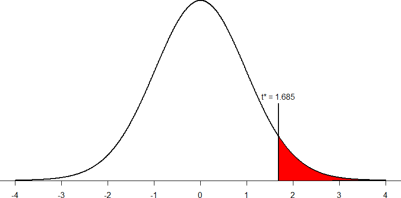
Figure 1. Critical region for one-tailed t-test at α = 0.05
Step 3: Calculate the Test Statistic
Now that the criteria are set, it is time to calculate the test statistic. The data obtained by the consultant found that the difference scores from time 1 to time 2 had a mean change of MD = 2.96 and a standard deviation of sD = 2.85. Using this information, plus the size of the sample (n = 40), we first calculate the standard error.
[latex]s_{M_D}=\frac{s_D}{\sqrt{n}}=\frac{2.85}{\sqrt{40}}=\frac{2.85}{6.32}=0.45[/latex]
Step 4: Make and Interpret the Decision
We have obtained a test statistic of ttest = 6.58 that we can compare to our previously established critical value of tcrit = 1.685. 6.85 is larger than 1.685, so ttest > tcrit and we reject the null hypothesis:
Reject H0. Based on the sample data from 40 workers, we can say that the intervention significantly improved job satisfaction (MD = 2.96, SD = 2.85) among the workers, t(39) = 6.85, p < 0.05.
Because this result was statistically significant, we will want to calculate Cohen’s d as an effect size using the same format as we did for the last t-test.
[latex]d=\frac{M_D}{s_D}={2.96}{2.85}=1.04[/latex]
So, now we can write our results in APA style one last time including effect size.
Reject H0. Based on the sample data from 40 workers, we can say that the intervention significantly improved job satisfaction (MD = 2.96, SD = 2.85) among the workers, t(39) = 6.85, p < 0.05, d = 1.04.
Confidence Intervals for Paired Samples t-Test
Confidence intervals for the paired-samples t-test are calculated the same way as they were calculated for the one-sample t-test.
Calculating a Confidence Interval for Paired-Samples t-Test
You will calculate an upper bound and a lower bound value for a confidence interval using the two-tailed critical value that corresponds to the level of confidence of interest.
[latex]CI_{UB}=M_D+t_{crit}\frac{s_D}{\sqrt{n}}[/latex]
[latex]CI_{LB}=M_D-t_{crit}\frac{s_D}{\sqrt{n}}[/latex]
To write out a confidence interval, you will use square brackets and put the lower bound, a comma, and the upper bound like this:
95% CI [LB value, UB value]
The 95% corresponds to the significance level used in calculating the confidence interval.
Assumptions are conditions that must be met in order for our hypothesis testing conclusion to be valid. It is important to remember that if the assumptions are not met then our hypothesis testing conclusion is not likely to be valid. Testing errors can still occur even if the assumptions for the test are met.
Recall that inferential statistics allow us to make inferences (decisions, estimates, predictions) about a population based on data collected from a sample. Recall also that an inference about a population is true only if the sample studied is representative of the population. A statement about a population based on a biased sample is not likely to be true. Now that we have been reminded of these things, let's look at our assumptions for a paired-samples t-test.
Assumption 1: Individuals in the sample were selected randomly and independently, so the sample is highly likely to be representative of the larger population.
- Random sampling ensures that each member of the population is equally likely to be selected.
- An independent sample is one which the selection of one member has no effect on the selection of any other.
Assumption 2: The distribution of sample differences is normal, because we drew the samples from a population that was normally distributed.
- This assumption is very important because we are estimating probabilities using the t- table - which provide accurate estimates of probabilities for events distributed normally.
Advantages & Disadvantages of using a repeated measures design
Advantages. Repeated measure designs reduce the probability of Type I errors when compared with independent sample designs because repeated measure designs reduce the probability that we will get a statistically significant difference that is due to an extraneous variable that differed between groups by chance (due to some other factor than the one in which we are interested).
Repeated measure designs are also more powerful (sensitive) than independent sample designs because two scores from each person are compared so each person serves as his or her own control group (we analyze the difference between scores). A special type of repeated measures design is known as the matched pairs design. If we are designing a study and suspect that there are important factors that could differ between our groups even if we randomly select and assign subjects, then we may use this type of design.
Because members of a matched-pair are similar to each other there is greater likelihood of our statistical test finding an “effect” when one person is present (power) in a repeated sample design as compared to a two-repeated sample design (in which subjects for two groups are picked randomly and independently - not matched on any traits).
Disadvantages. Repeated measure designs are very sensitive to outside influences and treatment influences. Outside Influences refers to factors outside of the experiment that may interfere with testing an individual across treatment/trials. Examples include mood or health or motivation of the individual participants. Think about it, if a participant tries really hard during the pretest but does not try very hard during the posttest, these differences can create problems later when analyzing the data.
Treatment Influences refers to the events that happen within the testing experience that interferes with how the data are collected. Three of the most common treatment influences are: 1. Practice effects, 2. Fatigue effects, and 3. Order effects.
Practice effect is present where participants perform a task better in later conditions because they have had a chance to practice it. Another type is a fatigue effect, where participants perform a task worse in later conditions because they become tired or bored. Order effects refer to differences in research participants’ responses that result from the order (e.g., first, second, third) in which the experimental materials are presented to them.
Imagine, for example, that participants judge the guilt of an attractive defendant and then judge the guilt of an unattractive defendant. If they judge the unattractive defendant more harshly, this might be because of his unattractiveness. But it could be instead that they judge him more harshly because they are becoming bored or tired. In other words, the order of the conditions is a confounding variable. The attractive condition is always the first condition and the unattractive condition the second. Thus any difference between the conditions in terms of the dependent variable could be caused by the order of the conditions and not the independent variable itself.
There is a solution to the problem of order effects, however, that can be used in many situations. It is counterbalancing, which means testing different participants in different orders. For example, some participants would be tested in the attractive defendant condition followed by the unattractive defendant condition, and others would be tested in the unattractive condition followed by the attractive condition. With three conditions, there would be six different orders (ABC, ACB, BAC, BCA, CAB, and CBA), so some participants would be tested in each of the six orders. With counterbalancing, participants are assigned to orders randomly, using the techniques we have already discussed. Thus random assignment plays an important role in related-samples designs just as in between-subjects designs. Here, instead of randomly assigning to conditions, they are randomly assigned to different orders of conditions. In fact, it can safely be said that if a study does not involve random assignment in one form or another, it is not an experiment.
Because the paired-samples design requires that each individual participate in more than one treatment, there is always the risk that exposure to the first treatment will cause a change in the participants that influences their scores in the second treatment that have nothing to do with the intervention. For example, if students are given the same test before and after the intervention the change in the posttest might be because the student got practice taking the test, not because the intervention was successful.
an index of dissimilarity or change between observations from the same individual across time, based on the measurement of a construct or attribute on two or more separate occasions.
two or more sets of study participants that are equivalent to one another with respect to certain relevant variables.
any change or improvement that results from practice or repetition of task items or activities.
a decline in performance on a prolonged or demanding research task that is generally attributed to the participant becoming tired or bored with the task.
the influence of the order in which treatments are administered, such as the effect of being the first administered treatment (rather than the second, third, and so forth).
