11 Independent-samples t-Test
Learning outcomes
In this chapter, you will learn how to:
- Identify when to use an independent-samples t-test
- Conduct an independent-samples t-test hypothesis test
- Evaluate effect size for an independent-samples t-test
- Identify the assumptions for conducting an independent-samples t-test
We have seen how to compare a single mean against a given value. While single sample techniques are used in real research, most research requires the comparison of at least two sets of data. Now, we will learn how to compare two separate means from two different groups to see if there is a difference between them. The process of testing hypotheses about two means is exactly the same as it is for testing hypotheses about a single mean, and the logical structure of the formula is the same as well. However, we will be adding a few extra steps this time to account for the fact that our data are coming from different sources.
The research designs used to obtain two sets of data can be classified into two general categories. If there’s no logical or meaningful way to link individuals across groups, or if there is no overlap between the groups, then we say the groups are independent and use the independent samples t-test (AKA between-subjects), the subject of this chapter. If they came from two time points with the same people, you know you are working with repeated measures data (the measurement literally was repeated) and will use a repeated measures (sometimes called a dependent samples or paired samples) t-test, which we will discuss in the next chapter. It is very important to keep these two tests separate and understand the distinctions between them because they assess very different questions and require different approaches to the data. When in doubt, think about how the data were collected and where they came from.
Research Questions about Independent Means
Remember that our research questions are always about the populations of interest, though we conduct the studies on samples. Thus, an independent samples t-test is truly designed to compare populations. If we want to know if two populations differ and we do not know the mean of either population, we take a sample from each and then conduct an independent sample t-test. Many research ideas in the behavioral sciences and other areas of research are concerned with whether or not two means are the same or different. Logically, we therefore say that these research questions are concerned with group mean differences. That is, on average, do we Group A to be higher or lower on some variable than Group B. In any time of research design looking at group mean differences, there are some key criteria we must consider: the groups must be mutually exclusive (i.e., you can only be part of one group at any given time) and the groups have to be measured on the same variable (i.e., you can’t compare personality in one group to reaction time in another group because those values would not be the same anyway).
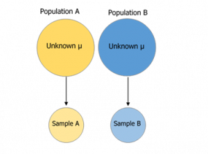
Figure 1. Collecting data from two different samples drawn from two different populations.
Let’s look at one of the most common and logical examples: testing a new medication. When a new medication is developed, the researchers who created it need to demonstrate that it effectively treats the symptoms they are trying to alleviate. The simplest design that will answer this question involves two groups: one group that receives the new medication (the “treatment” group) and one group that receives a placebo (the “control” group). Participants are randomly assigned to one of the two groups (remember that random assignment is the hallmark of a true experiment), and the researchers test the symptoms experienced by each person in each group after they received either the medication or the placebo. They then calculate the average symptoms in each group and compare them to see if the treatment group did better (i.e., had fewer or less severe symptoms) than the control group.
In this example, we had two groups (the independent variable): treatment and control. Membership in these two groups was mutually exclusive; each individual participant received either the experimental medication or the placebo. No one in the experiment received both, so there was no overlap between the two groups. Additionally, each group could be measured on the same variable: symptoms related to the disease or ailment being treated (the dependent variable). Because each group was measured on the same variable, the average scores in each group could be meaningfully compared. If the treatment was ineffective, we would expect that the average symptoms of someone receiving the treatment would be the same as the average symptoms of someone receiving the placebo (i.e., there is no difference between the groups). However, if the treatment was effective, we would expect fewer symptoms from the treatment group, leading to a lower group average.
Now, let’s look at an example using groups that already exist. A common, and perhaps salient, question is how students feel about their job prospects after graduation. Suppose that we have narrowed our potential choice of colleges down to two universities and, in the course of trying to decide between the two, we come across a survey that has data from each university on how students at those universities feel about their future job prospects. As with our last example, we have two groups: University A and University B, and each participant is in only one of the two groups. Because students at each university completed the same survey, they are measuring the same thing, so we can use an independent samples t-test to compare the average perceptions of students at each university to see if they are the same. If they are the same, then we should continue looking for other things about each university to help us decide on where to go. But, if they are different, we can use that information in favor of the university with higher job prospects.
As we can see, the grouping variable we use for an independent samples t-test can be a set of groups we create (as in the experimental medication example) or groups that already exist naturally (as in the university example). There are countless other examples of research questions relating to two group means, making the independent samples t-test one of the most widely used analyses around.
Hypotheses and Decision Criteria
The process of testing hypotheses using an independent samples t-test is the same as it was in the last two chapters, and it starts with stating our hypotheses and laying out the criteria we will use to test them.
The Null and Alternative Hypotheses
We still state the null and alternative hypotheses mathematically in terms of the population parameters and and then in words written out as statements answering the research questions as yes and no answers. Just like before, we need to decide if we are looking for directional or non-directional hypotheses. For a non-directional hypothesis test, our null hypothesis for an independent samples t-test is the same as all others: there is no difference. But instead of comparing a single 𝜇 to a numerical value, we are now comparing two populations, thus to 𝜇's. The means of the two groups are the same under the non-directional null hypothesis. Mathematically, this takes on two equivalent forms:
𝐻0: 𝜇1 = 𝜇2
or
𝐻0: 𝜇1 − 𝜇2 = 0
Both of these formulations of the null hypothesis tell us exactly the same thing: that the numerical values of the means are the same in both groups. This is more clear in the first formulation, but the second formulation also makes sense (any number minus itself is always zero) and helps us out a little when we get to the math of the test statistic. Either one is acceptable and you only need to report one. The written out version of both of them is also the same:
H0: There is no difference between the means of the two groups
Our alternative hypotheses are also unchanged. We simply replace the equal sign (=) with the inequality sign (≠):
𝐻𝐴: 𝜇1 ≠ 𝜇2
or
𝐻𝐴: 𝜇1 − 𝜇2 ≠ 0
Whichever format you chose for the null hypothesis should be the one you use for the alternative hypothesis (be consistent), and the interpretation of them is always the same:
HA: There is a difference between the means of the two groups
Notice that we are now dealing with two means instead of just one, so it will be very important to keep track of which mean goes with which population and, by extension, which dataset and sample data. We use subscripts to differentiate between the populations, so make sure to keep track of which is which. If it is helpful, you can also use more descriptive subscripts. To use the experimental medication example:
H0: There is no difference between the means of the treatment and control groups
𝐻0: 𝜇𝑡𝑟𝑒𝑎𝑡𝑚𝑒𝑛𝑡 = 𝜇𝑐𝑜𝑛𝑡𝑟𝑜𝑙
HA: There is a difference between the means of the treatment and control groups
𝐻𝐴: 𝜇𝑡𝑟𝑒𝑎𝑡𝑚𝑒𝑛𝑡 ≠ 𝜇𝑐𝑜𝑛𝑡𝑟𝑜𝑙
Degrees of Freedom for the Critical Value
Once we have our hypotheses laid out, we can set our criteria to test them using the same three pieces of information as before: significance level (α), directionality (one-tailed: left or right, or two-tailed), and degrees of freedom, which for an independent samples t-test are calculated a bit differently than before.
Calculating degrees of freedom for Independent Samples t-test
[latex]df=(n_1-1)+(n_2-1)[/latex]
Where n1 represents the sample size for group 1 and n2 represents the sample size for group 2. We have two separate groups, each with their own possible sample mean, so each has their own possible set of degrees of freedom (df = n -1).
This looks different than before, but it is just adding the individual degrees of freedom from each group (n – 1) together. Notice that the sample sizes, n, also get subscripts so we can tell them apart.
For an independent samples t-test, it is often the case that our two groups will have slightly different sample sizes, either due to chance or some characteristic of the groups themselves. Generally, this is not as issue, so long as one group is not massively larger than the other group. What is of greater concern is keeping track of which is which using the subscripts.
Computing the Test Statistic
The test statistic for our independent samples t-test takes on the same logical structure and format as our other t-tests: our observed effect minus our null hypothesis value, all divided by the standard error.
Calculating the test statistic for Independent Samples t-test
[latex]t_{test}=\frac{(M_1-M_2)-(𝜇_1-𝜇_2)}{s_{(M_1-M_2)}}[/latex]
M1 is the sample mean for group 1 and M2 is the sample mean for group 2. This looks like more work to calculate, but remember that our null hypothesis states that the quantity μ1 – μ2 = 0, so we can drop that out of the equation and are left with:
[latex]t_{test}=\frac{(M_1-M_2)}{s_{(M_1-M_2)}}[/latex]
Our standard error in the denominator is still estimated standard deviation (s) with a subscript denoting what it is the standard error of. Because we are dealing with the difference between two separate means, rather than a single mean, we put both means in the subscript. Calculating our standard error, as we will see next, is where the biggest differences between this t-test and other t-tests appears. However, once we do calculate it and use it in our test statistic, everything else goes back to normal. Our decision criteria is still comparing our obtained test statistic to our critical value, and our interpretation based on whether or not we reject the null hypothesis is unchanged as well.
Standard Error and Pooled Variance
Recall that the standard error is the average distance between any given sample mean and the center of its corresponding sampling distribution, and it is a function of the standard deviation of the population (either given or estimated) and the sample size. This definition and interpretation hold true for our independent samples t-test as well, but because we are working with two samples drawn from two populations, we have to first combine their estimates of standard deviation – or, more accurately, their estimates of variance – into a single value that we can then use to calculate our standard error.
The combined estimate of variance using the information from each sample is called the pooled variance and is denoted sp2; the subscript p serves as a reminder indicating that it is the pooled variance. The term “pooled variance” is a literal name because we are simply pooling or combining the information on variance – the Sum of Squares and Degrees of Freedom – from both of our samples into a single number. The result is a weighted average of the observed sample variances, the weight for each being determined by the sample size, and will always fall between the two observed variances.
Calculating the Pooled Variance and Standard Error for Independent Samples t-test
[latex]s_p^2=\frac{SS_1+SS_2}{df_1+df_2}[/latex]
Notice that pooled variance requires that we calculate the sum of squares for each sample and the degrees of freedom for each sample. Make sure you add before you divide when calculating pooled variance!
Once we have our pooled variance calculated, we can drop it into the equation for our standard error:
[latex]s_{(M_1-M_1)}=\sqrt{\frac{s_p^2}{n_1}+\frac{s_p^2}{n_2}}[/latex]
Unlike when calculating the pooled variance, here you want to make sure that you divide your fractions before you add!
Once again, although this formula may seem different than it was before, in reality it is just a different way of writing the same thing. Think back to the standard error options presented before, when our standard error was the square root of the just a single variance divided by a single sample size.
[latex]s_M=\sqrt{\frac{s^2}{n}}[/latex]
Looking at that, we can now see that, once again, we are simply adding together two pieces of information: no new logic or interpretation required. Once the standard error is calculated, it goes in the denominator of our test statistic, as shown above and as was the case in all previous chapters. Thus, the only additional step to calculating an independent samples t-statistic is computing the pooled variance. Let’s see an example in action.
Example: Movies and Mood
We are interested in whether the type of movie someone sees at the theater affects their mood when they leave. We decide to ask people about their mood as they leave one of two movies: a comedy (group 1, n1 = 35) or a horror film (group 2, n2 = 29). Our data are coded so that higher scores indicate a more positive mood. We have good reason to believe that people leaving the comedy will be in a better mood, so we use a one-tailed test at α = 0.05 to test our hypothesis.
Research Question: Will those who watch a comedy movie have a better mood than those who watch a horror film?
Step 1: State the Hypotheses
As always, we start with hypotheses:
H0: Those who watch the comedy will not have a better mood than those who watch the horror film
H0: μcomedy < μhorror
(Note that the null hypothesis includes both no difference (the equal sign) and a decrease in mood.)
HA: Those who watch the comedy will have a better mood than those who watch the horror film
HA: μcomedy > μhorror
Notice that we used labels to make sure that our data stay clear when we do our calculations later in this hypothesis test.
Step 2: Find the Critical Values
Just like before, we will need critical values, which come from our t-table. In this example, we have a one-tailed test at α = 0.05 and expect a positive answer (because we expect the difference between the means to be greater than zero). Our degrees of freedom for our independent samples t-test is just the degrees of freedom from each group added together:
[latex]df=(n_{comedy}-1)+(n_{horror}-1)=(35-1)+(29-1)=34+28=62[/latex]
From our t-table, we find that our critical value is tcrit = 1.671. Note that because 62 does not appear on the table, we use the next lowest value, which in this case is 60. Also, remember that since we are using a directional test, and looking for an increase or a positive change, that we keep the positive critical value. So, if we were to draw this out on a normal distribution, our critical region would be on the right side.
Step 3: Compute the Test Statistic
The data from our two groups are presented in the tables below. Table 1 shows the values for the Comedy group, and Table 2 shows the values for the Horror group. Values for both have already been placed in the Sum of Squares tables since we will need to use them for our further calculations. (See attached raw data set for additional practice.) Example Independent Samples t-test data (1)
|
Group 1: Comedy Film |
||
|
n |
M |
SS |
|
35 |
ΣX/n = 840/35 = 24 |
Σ(X − M)2=5061.60 |
Table 1. Raw scores and Sum of Squares for Group 1
|
Group 2: Horror Film |
||
|
n |
M |
SS |
| 29 | ΣX/n = 478.6/29 = 16.5 | Σ(X − M)2 = 3896.45 |
Table 2. Raw scores and Sum of Squares for Group 2.
These values have all been calculated and take on the same interpretation as they have since chapter 3 – no new computations yet. Before we move on to the pooled variance that will allow us to calculate standard error, let’s compute our standard deviation for each group; even though we will not use them in our calculation of the test statistic, they are still important descriptors of our data.
[latex]s_{comedy}^2=\frac{5061.60}{34}=148.87[/latex]
[latex]s_{comedy}=\sqrt{\frac{5061.60}{34}}=12.20[/latex]
and
[latex]s_{horror}^2=\frac{3896.45}{28}=139.16[/latex]
[latex]s_{horror}=\sqrt{\frac{3896.45}{28}}=11.80[/latex]
Now we can move on to our new calculation, the pooled variance, which is the Sums of Squares that we calculated from our table and the degrees of freedom, which is n – 1, for each group.
[latex]s_p^2=\frac{SS_{comedy}+SS_{horror}}{df_{comedy}+df_{horror}}[/latex]
[latex]s_p^2=\frac{5061.60+3896.45}{34+28}=\frac{8958.05}{62}=144.48[/latex]
As you can see, if you follow the regular process of calculating standard deviation using the Sum of Squares table, finding the pooled variance is very easy.
Now we can use the pooled variance calculated above to calculate our standard error, the last step before we can find our test statistic.
[latex]s_{M_1-M_2}=\sqrt{\frac{s_p^2}{n_{comedy}}+\frac{s_p^2}{n_{horror}}}[/latex]
[latex]s_{M_1-M_2}=\sqrt{\frac{144.48}{35}+\frac{144.48}{29}}=\sqrt{4.13+4.98}=\sqrt{9.11}=3.02[/latex]
Finally, we can use our standard error and the means we calculated earlier to compute our test statistic. Because the null hypothesis value of μ1 – μ2 is 0, we will leave that portion out of the equation for simplicity.
[latex]t_{test}=\frac{M_{comedy}-M_{horror}}{s_{M_1-M_2}}[/latex]
[latex]t_{test}=\frac{24.00-16.50}{3.02}=\frac{7.50}{3.02}=2.48[/latex]
The process of calculating our test statistic ttest = 2.48 followed the same sequence of steps as before: use raw data to compute the mean and sum of squares (this time for two groups instead of one), use the sum of squares and degrees of freedom to calculate standard error (this time using pooled variance instead of standard deviation), and use that standard error and the observed means to get ttest.
Now we can move on to the final step of the hypothesis testing procedure.
Step 4: Make and Interpret the Decision
Our test statistic has a value of ttest = 2.48, and in step 2 we found that the critical value is tcrit = 1.671. 2.48 > 1.671, so we reject the null hypothesis. We can now write our decision up in APA style. Notice that we use our combined degrees of freedom in our inferential statistics in the statement below.
Reject H0. The average mood after watching a comedy movie (M = 24.00, SD = 12.20) is significantly better than the average mood after watching a horror movie (M = 16.50, SD = 11.80), t(62) = 2.48, p < .05.
However, we shouldn't stop there. Since we found an effect, we want to make sure to calculate effect size next.
Effect Sizes and Confidence Intervals
We have seen in previous chapters that even a statistically significant effect needs to be interpreted along with an effect size to see if it is practically meaningful. We have also seen that our sample means, as a single estimate, are not perfect and would be better represented by a range of values that we call a confidence interval. As with all other topics, this is also true of our independent samples t-tests.
Our effect size for the independent samples t-test is still Cohen’s d, and it is still just our observed effect or difference divided by the standard deviation. Remember that standard deviation is just the square root of the variance, and because we work with pooled variance in our test statistic, we will use the square root of the pooled variance as our denominator in the formula for Cohen’s d.
Calculating Cohen's d for Independent Samples t-test
[latex]d=\bigg |\frac{M_1-M_2}{\sqrt{s_p^2}}\bigg |[/latex]
For our example above, we can calculate the effect size to be:
[latex]d=\bigg |\frac{24.00-16.50}{\sqrt{144.48}}\bigg |=\bigg |\frac{7.50}{12.02}\bigg |=0.62[/latex]
We interpret this using the same guidelines as before, so we would consider this a medium effect. And, now we should add this to our sentence from above.
The average mood after watching a comedy movie (M = 24.00, SD = 12.20) is significantly better than the average mood after watching a horror movie (M = 16.50, SD = 11.80), t(62) = 2.48, p < .05, d = 0.62.
Confidence Intervals
Our confidence intervals also take on the same form and interpretation as they have in the past. The value we are interested in is the difference between the two means, so our single estimate is the value of one mean minus the other, or M1 - M2 . Just like before, this is our observed effect and is the same value as the one we place in the numerator of our test statistic. We calculate this value then place the margin of error – still our two-tailed critical value times our standard error – above and below it.
Calculating Confidence Interval for Independent Samples t-test
[latex]CI_{upper}=(M_1-M_2)+t_{crit}\sqrt{\frac{s_p^2}{n_1}+\frac{s_p^2}{n_2}}[/latex]
[latex]CI_{lower}=(M_1-M_2)-t_{crit}\sqrt{\frac{s_p^2}{n_1}+\frac{s_p^2}{n_2}}[/latex]
Because our hypothesis testing example used a one-tailed test, it would be inappropriate to calculate a confidence interval on those data (remember that we can only calculate a confidence interval for a two-tailed test because the interval extends in both directions). Let’s say we find summary statistics on the average life satisfaction of people from two different towns and want to create a confidence interval to see if the difference between the two might actually be zero.
Our sample data are M1 =28.65, s1 = 12.40, n1 = 40 and M2 = 25.40, s2 = 15.68, n2 = 42. At face value, it looks like the people from the first town have higher life satisfaction (28.65 vs. 25.40), but it will take a confidence interval (or complete hypothesis testing process) to see if that is true or just due to random chance.
First, we want to calculate the difference between our sample means, which is 28.65 – 25.40 = 3.25.
Next, we need a critical value from our t-table. If we want to test at the normal 95% level of confidence, then our sample sizes will yield degrees of freedom equal to (40-1) + (42-1) = 40 + 42 – 2 = 80. From our table, that gives us a critical value of tcrit = 1.990.
Finally, we need our standard error. Recall that our standard error for an independent samples t-test uses pooled variance, which requires the Sum of Squares and degrees of freedom. Up to this point, we have calculated the Sum of Squares using raw data, but in this situation, we do not have access to it. So, what are we to do?
If we have summary data like standard deviation and sample size, it is very easy to calculate the pooled variance another version of the formula.
Calculating Pooled Variance from Sample Standard Deviations
[latex]s_p^2=\frac{(n_1-1)s_1^2+(n_2-1)s_2^2}{n_1+n_2-2}[/latex]
If s1 = 12.40, then s12 = 12.40*12.40 = 153.76, and if s2 = 15.68, then s22 = 15.68*16.68 = 245.86. With n1 = 40 and n2 = 42, we are all set to calculate the pooled variance.
[latex]s_p^2=\frac{(40-1)(153.76)+(42-1)(245.86)}{40+42-2}=\frac{(39)(153.76)+(41)(245.86)}{80}[/latex]
[latex]s_p^2=\frac{5996.64+10080.36}{80}=\frac{16077.00}{80}=200.96[/latex]
Now we can plug sp2 = 200.96, n1 = 40, and n2 = 42nd, in to our standard error equation.
[latex]s_{M_1-M_2}=\sqrt{\frac{s_p^2}{n_1}+\frac{s_p^2}{n_2}}=\sqrt{\frac{200.96}{40}+\frac{200.96}{42}}=\sqrt{5.02+4.78}=\sqrt{9.89}=3.14[/latex]
All of these steps are just slightly different ways of using the same formula, numbers, and ideas we have worked with up to this point. Once we get out standard error, it’s time to build our confidence interval.
95% CI = 3.25 + 1.990(3.14)
95% CIupper = 3.25 + 1.990(3.14) = 3.25 + 6.25 = 9.50
95% CIlower = 3.25 - 1.990(3.14) = 3.25 - 6.25 = -3.00
CI95 [-3.00, 9.50]
Our confidence interval, as always, represents a range of values that would be considered reasonable or plausible based on our observed data. In this instance, our interval (-3.00, 9.50) does contain zero. Thus, even though the means look a little bit different, it may very well be the case that the life satisfaction in both of these towns is the same. Proving otherwise would require more data.
Homogeneity of Variance
Before wrapping up the coverage of independent samples t-tests, there is one other important topic to cover. Using the pooled variance to calculate the test statistic relies on an assumption known as homogeneity of variance AKA equality of variances AKA homoscedasticity. In statistics, an assumption is some characteristic that we assume is true about our data, and our ability to use our inferential statistics accurately and correctly relies on these assumptions being true. If these assumptions are not true, then our analyses are at best ineffective (e.g., low power to detect effects) and at worst inappropriate (e.g., too many Type I errors). A detailed coverage of assumptions is beyond the scope of this textbook, but it is important to know that they exist for all analyses.
For the current hypothesis test, one important assumption is homogeneity of variance. This is fancy statistical talk for the idea that the true population variance for each group is the same and any difference in the observed sample variances is due to random chance. (If this sounds eerily similar to the idea of testing the null hypothesis that the true population means are equal, that’s because it is exactly the same!) This notion allows us to compute a single pooled variance that uses our easily calculated degrees of freedom. If the assumption is shown to not be true, then we have to use a very complicated formula to estimate the proper degrees of freedom. There are formal tests to assess whether or not this assumption is met, but we will not discuss them here., however most statistical programs will run these assumption checks for us.
Many statistical programs incorporate the test of homogeneity of variance automatically and can report the results of the analysis assuming it is true or assuming it has been violated. You can easily tell which is which by the degrees of freedom: the corrected degrees of freedom (which is used when the assumption of homogeneity of variance is violated) will have decimal places. Fortunately, the independent samples t-test is very robust to violations of this assumption (an analysis is “robust” if it works well even when its assumptions are not met), which is why we do not bother going through the tedious work of testing and estimating new degrees of freedom by hand.
Review: Statistical Power
There are three factors that can affect statistical power:
- Sample size: Larger samples provide greater statistical power
- Effect size: A given design will always have greater power to find a large effect than a small effect (because finding large effects is easier)
- Type I error rate: There is a relationship between Type I error and power such that (all else being equal) decreasing Type I error will also decrease power.
We can see this through simulation. First let’s simulate a single experiment, in which we compare the means of two groups using a standard t-test. We will vary the size of the effect (specified in terms of Cohen’s d), the Type I error rate, and the sample size, and for each of these we will examine how the proportion of significant results (i.e. power) is affected. Figure 1 shows an example of how power changes as a function of these factors.
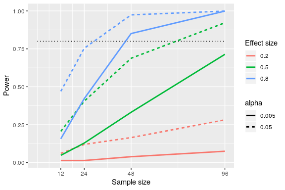
Figure 1: Results from power simulation, showing power as a function of sample size, with effect sizes shown as different colors, and alpha shown as line type. The standard criterion of 80 percent power is shown by the dotted black line.
This simulation shows us that even with a sample size of 96, we will have relatively little power to find a small effect (d=0.2) with α=0.005. This means that a study designed to do this would be futile – that is, it is almost guaranteed to find nothing even if a true effect of that size exists.
There are at least two important reasons to care about statistical power. First, if you are a researcher, you probably don’t want to spend your time doing futile experiments. Running an underpowered study is essentially futile, because it means that there is a very low likelihood that one will find an effect, even if it exists. Second, it turns out that any positive findings that come from an underpowered study are more likely to be false compared to a well-powered study. Fortunately, there are tools available that allow us to determine the statistical power of an experiment. The most common use of these tools is in planning an experiment, when we would like to determine how large our sample needs to be in order to have sufficient power to find our effect of interest.
Assumptions of independent-samples t-tests
Assumptions are conditions that must be met in order for our hypothesis testing conclusion to be valid. [Important: If the assumptions are not met then our hypothesis testing conclusion is not likely to be valid. Testing errors can still occur even if the assumptions for the test are met.]
Recall that inferential statistics allow us to make inferences (decisions, estimates, predictions) about a population based on data collected from a sample. Recall also that an inference about a population is true only if the sample studied is representative of the population. A statement about a population based on a biased sample is not likely to be true.
Assumption 1: Individuals in the sample were selected randomly and independently, so the sample is highly likely to be representative of the larger population.
- Random sampling ensures that each member of the population is equally likely to be selected.
- An independent sample is one in which the selection of one member has no effect on the selection of any other.
Assumption 2: The distribution of sample mean differences is a normal, because we drew the samples from a population that was normally distributed or we drew large enough samples that the law of large numbers has worked in our favor.
- This assumption is very important because we are estimating probabilities using the t- table, which provide accurate estimates of probabilities for events distributed normally.
Assumption 3: Sampled populations have equal variances or have homogeneity of variance as discussed above.
a research design that uses a separate group of participants for each treatment condition
the statistical assumption of equal variance, meaning that the average squared distance of a score from the mean is the same across all groups sampled in a study.
