10 One-sample t-Test
Learning outcomes
In this chapter, you will learn how to:
- Identify when to use t statistic instead of a z-score hypothesis test
- Conduct a one-sample hypothesis test
- Evaluate effect size
- Calculate a confidence interval to estimate a population parameter
In the last unit, we made a big leap from basic descriptive statistics into full hypothesis testing and inferential statistics. In this unit, we will be learning new tests, each of which is just a small adjustment on the test before it.
The procedures for testing hypotheses described up to this point were necessary for what comes next, but these procedures involved comparing a group of scores to a known population. In real research practice, we often compare two or more groups of scores to each other, without any direct information about populations. For example:
- Comparing the intelligence scores (IQ) of one sample to standardized IQ norms based on hypothesized population values.
- Comparing anxiety scores for a group of patients before and after psychotherapy or number of familiar versus unfamiliar words recalled in a memory experiment.
- Comparing scores on a cognitive test for a group of participants experiencing sleep deprivation and a group of participants who slept normally.
- Comparing scores on self-esteem test scores for a group of 10-year-old girls to a group of 10-year-old boys.
It is more common in psychology to only have information from samples and know nothing about the population that the samples are supposed to come from. In particular, the researcher does not know the variance of the populations involved. In this chapter, we will learn the solution to the problem of the unknown population variance.
In this chapter, we will learn about the first of three t-tests.
The t-statistic for one-sample
Last chapter, we were introduced to hypothesis testing using the z-statistic for sample means. This was a useful way to link the material and ease us into the new way to looking at data, but it isn’t a very common test because it relies on knowing the population standard deviation, σ, which is rarely going to be the case. Instead, we will estimate that parameter σ using the sample statistics in the same way that we estimate μ using M.
Calculating a t-Statistic
[latex]t=\frac{M-μ}{s_M}[/latex]
Notice that t looks almost identical to z; this is because they test the exact same thing: the value of a sample mean compared to what we expect of the population. The only difference is that the standard error is now denoted as sM to indicate that we use the sample statistic for standard deviation, s, instead of the population parameter σ. We call the standard error using s, the estimated standard error of the mean.
Calculating a estimated standard error
[latex]s_M=\frac{s}{\sqrt{n}}[/latex]
Setting up for step 2
In order to find the critical region for a t-test we must use degrees of freedom (df). We previously learned that the formula for sample standard deviation and population standard deviation differ by one key factor: the denominator for the parameter is N but the denominator for the statistic is n – 1, also known as degrees of freedom, df. As we learned earlier, degrees of freedom gets its name because it is the number of scores in a sample that are “free to vary”. The idea is that when finding the variance we must first know the mean. If we know the mean and all but one of the scores in a sample, we can figure out the one we do not know with a little math. In this situation the degrees of freedom is the number of scores minus 1.
Because we are using a new equation, we can no longer use the standard normal distribution and the z-table to find our critical values. For t-tests, we will use the t-distribution and t-table to find these values.
The t-distribution, like the standard normal distribution, is symmetric and normally distributed with a mean of 0. However, because the calculation of estimated standard error uses degrees of freedom, there will be a different t-distribution for every degree of freedom.
Figure 1 shows four curves: a normal distribution curve labeled z, and three t-distribution curves for 2, 10, and 30 degrees of freedom. Remember, degrees of freedom refers to the maximum number of logically independent values, which are values that have the freedom to vary, in the sample. Two things should stand out: First, for lower degrees of freedom (e.g., 2), the tails of the distribution are much fatter, meaning a larger proportion of the area under the curve falls in the tail. This means that we will have to go farther out into the tail to cut off the portion corresponding to 5% or α = 0.05, which will, in turn, lead to higher critical (rejection) values. Second, as the degrees of freedom increase, we get closer and closer to the z curve. Even the distribution with df = 30, corresponding to a sample size of just 31 people, is nearly indistinguishable from z. In fact, a t-distribution with infinite degrees of freedom (theoretically, of course) is exactly the standard normal distribution. Because of this, the bottom row of the t-table is equivalent to the critical values for z-tests at the specific significance levels. Even though these curves are very close, it is still important to use the correct table and critical values, because small differences can add up quickly.
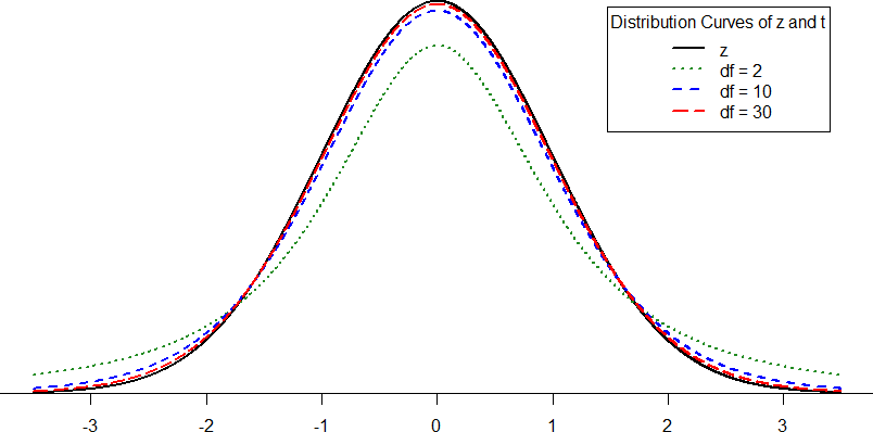
Figure 1. Distributions comparing effects of degrees of freedom
The t-distribution table lists critical values for one- and two-tailed tests at several levels of significance arranged into columns. The rows of the t-table list degrees of freedom up to df = 120 in order to use the appropriate distribution curve. It does not, however, list all possible degrees of freedom in this range, because that would take too many rows. Greater than df = 30, the rows jump in increments of 10. If a problem requires you to find critical values and the exact degrees of freedom is not listed, you always round down to the next smallest number. For example, if you have 48 people in your sample, the degrees of freedom are n – 1 = 48 – 1 = 47; however, 47 doesn’t appear on our table, so we round down and use the critical values for df = 40, even though 50 is closer. We do this because it avoids inflating Type I Error (false positives, see chapter 9) by using criteria that are too lax.
Hypothesis Testing with t
Hypothesis testing with the t-statistic works exactly the same way as z-tests did, following the four-step process of 1) Stating the Hypotheses, 2) Finding the Critical Value(s), 3) Computing the Test Statistic, and 4) Making and Interpreting the Decision. We will work though an example: let’s say that you move to a new city and find a an auto shop to change your oil. Your old mechanic did the job in about 30 minutes (though you never paid close enough attention to know how much that varied), and you suspect that your new shop takes much longer. After 4 oil changes, you think you have enough evidence to demonstrate this.
Step 1: State the Hypotheses
Our hypotheses for one-sample t-tests are identical to those we used for z-tests. We still state the null and alternative hypotheses mathematically in terms of the population parameter and written out. First, we need to decide if we are looking for directional or non-directional hypotheses. For our example, you are wanting to know if the new shop takes longer to change your oil which would be a directional hypothesis. The hypotheses would be stated as:
H0: This shop does not take longer to change the oil than your old mechanic
H0: μ < 30
HA: This shop takes longer to change oil than your old mechanic
HA: μ > 30
Step 2: Find the Critical Values
As noted above, our critical values still delineate the area in the tails under the curve corresponding to our chosen level of significance. For this example we will use α = 0.05, and because we suspect a direction of effect, we have a one-tailed test. To find our critical values for t, we need to add one more piece of information: the degrees of freedom. For this example:
df = n – 1 = 4 – 1 = 3
Going to a t-table, we find the column corresponding to our one-tailed significance level and find where it intersects with the row for 3 degrees of freedom. As shown in Figure 2: our critical value is tcrit = 2.353.
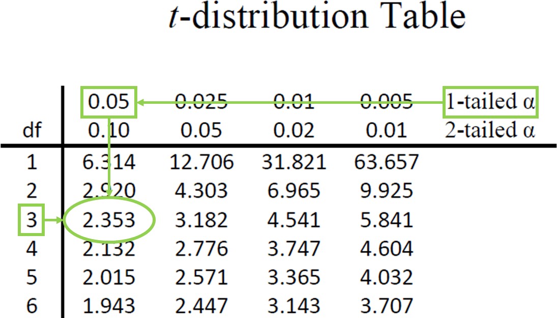
Figure 2. t-table
We can then shade this region on our t-distribution to visualize our critical region.
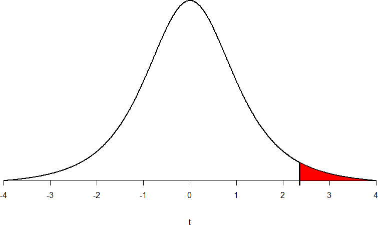
Figure 3. Critical Region for tcrit = 2.353.
Step 3: Compute the Test Statistic
The four wait times you experienced for your oil changes at the new shop were 46 minutes, 58 minutes, 40 minutes, and 71 minutes. We will use these to calculate M.
[latex]M=\frac{ΣX}{n}=\frac{46+58+40+71}{4}=\frac{215}{4}=53.75[/latex]
Next, we will need to calculate the standard deviation so we can calculate the ttest. We will do this through both the definitional and computational methods outlined in Chapter 5.
|
X |
X–M |
(X–M)2 |
|
46 |
-7.75 |
60.06 |
|
58 |
4.25 |
18.06 |
|
40 |
-13.75 |
189.06 |
|
71 |
17.25 |
297.56 |
|
Σ = 215 |
Σ = 0 |
Σ = 564.74 |
Table 1. Sum of Squares (SS) table using the definitional method
[latex]s=\sqrt{\frac{SS}{df}}=\sqrt{\frac{564.74}{4-1}}=\sqrt{\frac{564.74}{3}}=\sqrt{188.25}=13.72[/latex]
|
X |
X2 |
|
46 |
2116 |
|
58 |
3364 |
|
40 |
1600 |
|
71 |
5041 |
|
Σ = 215 |
Σ = 12121 |
Table 2. Sum of Squares Table using the definitional method
[latex]SS=ΣX^2-\frac{(ΣX)^2}{n}=12121-\frac{215*215}{4}=12121-\frac{46225}{4}[/latex]
[latex]SS=12121-11556.25=564.75[/latex]
[latex]s=\sqrt{\frac{SS}{df}}=\sqrt{\frac{564.75}{4-1}}=\sqrt{\frac{564.75}{3}}=\sqrt{188.25}=13.72[/latex]
Notice that once again, the two routes get the same standard deviation. Now, we will take this value and plug it in to the formula for estimated standard error.
[latex]s_M=\frac{s}{\sqrt{n}}=\frac{13.72}{\sqrt{4}}=\frac{13.72}{2}=6.86[/latex]
And, finally, we put the standard error, sample mean, and null hypothesis value into the formula for our test statistic ttest.
[latex]t_{test}=\frac{M-μ}{s_M}=\frac{53.75-30}{6.86}=\frac{23.75}{6.86}=3.46[/latex]
Step 4: Make and Interpret the Decision
Now that we have our critical value and test statistic, we can make our decision using the same criteria we used for a z-test. Our t-test was t = 3.46 and our critical value was tcrit = 2.353: ttest > tcrit, so we reject the null hypothesis and interpret our results by writing the following sentence.
Based on our four oil changes, the new mechanic takes significantly longer on average (M = 53.75, SD = 13.72) to change oil than our old mechanic, t(3) = 3.46, p < .05.
Notice that we also include the degrees of freedom in parentheses next to t so that the reader knows how much of an estimate our t-statistic is. Finally, because we found a significant result, we need to calculate an effect size, which is still Cohen’s d, but now we use s in place of σ.
[latex]d=\bigg |\frac{M-𝜇}{s}\bigg |[/latex]
[latex]d=\bigg |\frac{53.75-30}{13.72}\bigg |=\bigg |\frac{23.75}{13.72}\bigg |=|1.73|=1.73[/latex]
| d | Interpretation |
|---|---|
| 0.0 - 0.2 | negligible |
| 0.2 - 0.5 | small |
| 0.5 - 0.8 | medium |
| 0.8 + | large |
Table 3. Interpretation of Cohen's d
We can compare to Table 3 like we did in the last chapter to figure out the size of the effect. This is a large effect. Now, we can rewrite our sentence to include this additional information.
Based on our four oil changes, the new mechanic takes significantly longer on average (M = 53.75, SD = 13.72) to change oil than our old mechanic, t(3) = 3.46, p < .05., d = 1.73.
Confidence Intervals
Up to this point, we have learned how to estimate the population parameter for the mean using sample data and a sample statistic. From one point of view, this makes sense: we have one value for our parameter so we use a single value to estimate it. However, we have seen that all statistics have sampling error and that the value we find for the sample mean will vary based on the people in our sample, simply due to random chance. Thinking about estimation from this perspective, it would make more sense to take that error into account rather than relying on a single estimate. To do this, we calculate what is known as a confidence interval.
A confidence interval starts with a single estimate then creates a range of scores considered plausible based on our standard deviation, our sample size, and the level of confidence with which we would like to estimate the parameter. This range, which extends equally in both directions away from the original estimate, is called the margin of error. We calculate the margin of error by multiplying our two-tailed critical values by our standard error.
Calculating Margin of Error (MoE) for a Confidence Interval
[latex]MoE=t_{crit}\frac{s}{\sqrt{n}}[/latex]
One important consideration when calculating the margin of error is that it can only be calculated using the critical value for a two-tailed test. This is because the margin of error moves away from the original estimate in both directions, so a one- tailed value does not make sense.
The critical value we use will be based on a chosen level of confidence, which is equal to 1 – α. Thus, a 95% level of confidence corresponds to α = 0.05. In other words, at the 0.05 level of significance, we create a 95% Confidence Interval.
Once we have our margin of error calculated, we add it to our original estimate for the mean to get an upper bound to the confidence interval and subtract it from the original estimate for the mean to get a lower bound for the confidence interval.
Calculating a Confidence Interval
You will calculate an upper bound and a lower bound value for a confidence interval.
[latex]CI_{UB}=M+t_{crit}\frac{s}{\sqrt{n}}[/latex]
[latex]CI_{LB}=M-t_{crit}\frac{s}{\sqrt{n}}[/latex]
To write out a confidence interval, you will use square brackets and put the lower bound, a comma, and the upper bound like this:
95% CI [LB value, UB value]
The 95% corresponds to the significance level used in calculating the confidence interval.
Let’s see what this looks like with some actual numbers by taking our oil change data and using it to create a 95% confidence interval estimating the average length of time it takes at the new mechanic. We already found that our average was M = 53.75 and our standard error was sM = 6.86.
We also found a critical value to test our hypothesis, but remember that we were testing a one-tailed hypothesis, so that critical value won’t work. To see why that is, look at the column headers on the t- table. The column for one-tailed α = 0.05 is the same as a two-tailed α = 0.10. If we used the old critical value, we’d actually be creating a 90% confidence interval (1.00-0.10 = 0.90, or 90%). To find the correct value, we use the column for two- tailed α = 0.05 and, again, the row for 3 degrees of freedom, to find tcrit = +3.182.
Now we have all the pieces we need to construct our confidence interval.
95% CI = 53.75 ± 3.182(6.86)
upper bound = 53.75 + 3.182(6.86)
UB = 53.75 + 21.83 = 75.58
lower bound = 53.75 − 3.182(6.86)
LB = 53.75 − 21.83 = 31.92
95% CI [31.92, 75.58]
So we find that our 95% confidence interval runs from 31.92 minutes to 75.58 minutes, but what does that actually mean? The range (31.92, 75.58) represents values of the mean that we consider reasonable or plausible based on our observed data. It includes our single estimate of the mean, M = 53.75, in the center, but it also has a range of values that could also have been the case based on what we know about how much these scores vary (i.e. our standard error).
It is very tempting to also interpret this interval by saying that we are 95% confident that the true population mean falls within the range (31.92, 75.58), but this is not true. The reason it is not true is that phrasing our interpretation this way suggests that we have firmly established an interval and the population mean does or does not fall into it, suggesting that our interval is firm and the population mean will move around. However, the population mean is an absolute that does not change; it is our interval that will vary from data collection to data collection, even taking into account our standard error. The correct interpretation, then, is that we are 95% confident that the range [31.92, 75.58] brackets the true population mean. This is a very subtle difference, but it is an important one.
Interpreting Confidence Intervals
Confidence intervals are notoriously confusing, primarily because they don’t mean what we might intuitively think they mean. If I tell you that I have computed a “95% confidence interval” for my statistic, then it would seem natural to think that we can have 95% confidence that the true parameter value falls within this interval. However, as we will see throughout the course, concepts in statistics often don’t mean what we think they should mean. In the case of confidence intervals, we can’t interpret them in this way because the population parameter has a fixed value – it either is or isn’t in the interval, so it doesn’t make sense to talk about the probability of that occurring. Jerzy Neyman, the inventor of the confidence interval, said:
“The parameter is an unknown constant and no probability statement concerning its value may be made.”(Neyman 1937)
Instead, we have to view the confidence interval procedure from the same standpoint that we viewed hypothesis testing: As a procedure that in the long run will allow us to make correct statements with a particular probability. Thus, the proper interpretation of the 95% confidence interval is that it is an interval that will contain the true population mean 95% of the time.
a measure of the variability between a sample mean and population mean based on a specific sample size, n.
Degrees of freedom = df = n – 1, measures the number of scores that are free to vary when computing SS for sample data. The value of df also describes how well a t statistic estimates a z-score. (as discussed in Unit 3).
A range of values for a population parameter that is estimated from a sample with a preset, fixed probability (known as the confidence level) that the range will contain the true value of the parameter. The width of the confidence interval provides information about the precision of the estimate, such that a wider interval indicates relatively low precision and a narrower interval indicates relatively high precision.
A value that gives the frequency that a given confidence interval contains the true value of the population parameter being estimated. Usually 95% or 99% is most commonly used.
