Understanding Algorithms

To embark on a journey into the realm of Machine Learning (ML), one must grasp the fundamental concepts of algorithms and models, as they serve as the bedrock upon which predictive and analytical capabilities are built.  At its core, an algorithm is a set of step-by-step instructions that a machine follows to perform a specific task. In the context of ML, algorithms are the engines of learning—they enable systems to recognize patterns, make predictions, or generate insights from data.

Key Aspects of Algorithms

• Task-Specificity: Different algorithms are designed for different tasks. For instance, a decision tree algorithm is suitable for classification, while linear regression is apt for predicting numerical values.
• Complexity: Algorithms vary in complexity, from simple linear models to sophisticated deep neural networks. The complexity is often tailored to the intricacy of the problem at hand.
• Learning Paradigm: Supervised, unsupervised, or semi-supervised algorithms adhere to specific learning paradigms, governing how they process and learn from data.

Task-Specificity

As noted above, the choice of algorithm depends on the task at hand—whether it’s predicting outcomes, classifying data, or uncovering patterns in a dataset.  Some common types of algorithms include Linear Regression, Decision Trees, K-Means Clustering, and Neural Networks.   We will look at each of these in turn.

Linear Regression

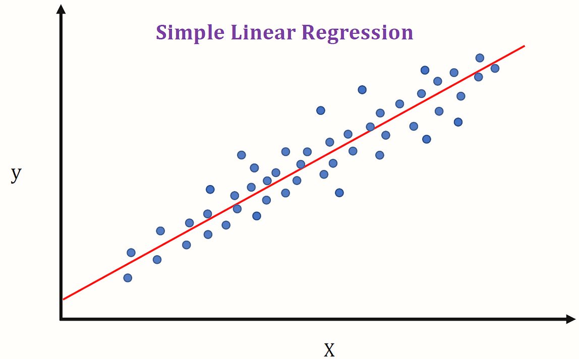Linear regression is a fundamental supervised learning algorithm used in AI/ML for predicting a continuous target variable based on one or more independent features. It assumes a linear relationship between the input features and the target variable. The goal is to find the best-fit line that minimizes the difference between the predicted and actual values. Here’s an overview of how linear regression algorithms work:

Model Representation: In simple linear regression, there is one independent variable (feature) denoted as X and one dependent variable (target) denoted as Y.  The relationship is represented by the equation:

[latex]Y={\beta_0}+{\beta_0} \cdot X+\varepsilon[/latex]

where [latex]\beta_0[/latex] is the y-intercept, [latex]\beta_1[/latex] Is the slope, and [latex]\varepsilon[/latex] represents the error term.

Training the Model:  The model is trained by adjusting the parameters [latex]\beta_0[/latex] and [latex]\beta_1[/latex] using optimization techniques such as gradient descent. The goal is to find the values that minimize the error, which quantifies the difference between predictions and actual values.

Making Predictions:  Once trained, the linear regression model can make predictions for new data points by plugging in the values of the independent variable into the learned equation.

Assumptions of Linear Regression:

1. Linearity:  The relationship between the independent and dependent variables is assumed to be linear.
2. Independence:  Observations are assumed to be independent of each other.
3. Homoscedasticity:  The variance of the residuals (errors) is assumed to be constant across all levels of the independent variable.
4. Normality of Residuals:  The residuals are assumed to follow a normal distribution.

Linear regression is widely used for tasks such as predicting house prices, stock prices, and other continuous variables where a linear relationship is assumed to exist between features and the target variable.

Decision-Tree Algorithms

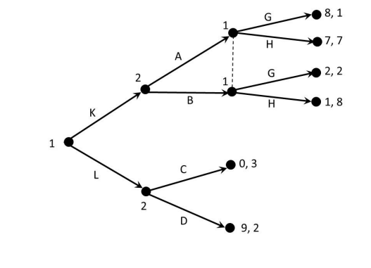
Decision trees are powerful and versatile algorithms used in AI/ML for both classification and regression tasks. They model decision-making processes by recursively splitting the dataset into subsets based on the values of features. The goal is to create a tree structure that guides the algorithm in making decisions or predictions. Decision trees are particularly useful because they can handle both categorical and numerical features, making them suitable for a wide range of datasets. Each internal node of the tree represents a decision based on a specific feature, while the leaf nodes represent the final prediction or classification.

One of the main advantages of decision trees is their interpretability. Since the decision-making process is represented as a series of if-else conditions, it is easy to understand how the algorithm arrived at a particular prediction. This interpretability is crucial in domains where explainability is important, such as healthcare or finance.

Moreover, decision trees are capable of handling missing values and outliers by utilizing surrogate splits. These surrogate splits allow the algorithm to make decisions even when certain features are missing or contain outliers, making them robust in real-world scenarios.

Another benefit of decision trees is their ability to handle both binary and multi-class classification problems. By using different splitting criteria, such as Gini impurity or information gain, decision trees can effectively separate data points into different classes.

Furthermore, decision trees can be combined to create ensemble methods such as random forests or gradient boosting. These ensemble methods improve the accuracy and generalization of the model by aggregating the predictions of multiple decision trees.

However, decision trees are prone to overfitting, especially when the tree becomes too deep or complex. Overfitting occurs when the model memorizes the training data instead of learning general patterns, leading to poor performance on unseen data. To mitigate overfitting, techniques such as pruning or limiting the depth of the tree can be applied.

Here’s an overview of how decision-tree algorithms work:

Decision Tree Construction:

• Root Node:  The algorithm begins by selecting the feature that best splits the dataset into subsets. This feature becomes the root node of the tree.
• Splitting Criteria: The decision to split is based on a splitting criterion, often measured by metrics like Gini impurity (for classification) or mean squared error (for regression).  The Gini impurity measures the degree or probability of a particular variable being wrongly classified when it is randomly chosen. The splitting criterion aims to minimize the impurity or error in each subset.
• Recursive Splitting: The dataset is divided into subsets based on the chosen feature’s values. This process is repeated recursively for each subset, creating branches and nodes in the tree.
• Stopping Criteria: The recursion stops when a predefined stopping criterion is met. This could include reaching a maximum depth, achieving a minimum number of samples in a node, or no further improvement in the chosen criterion.

Decision-Making:

• Leaf Nodes: Terminal nodes or leaf nodes represent the final decision or prediction. For classification, each leaf node corresponds to a class label. For regression, it contains the predicted continuous value.
• Traversal: To make a decision or prediction for a new instance, it traverses the tree from the root, following the splits based on the feature values until it reaches a leaf node.

Advantages of Decision Trees:

• Interpretability:  Decision trees are easy to interpret and visualize, making them useful for understanding decision logic.
• Handling Non-Linearity: They can capture non-linear relationships in the data without explicitly specifying complex mathematical functions.
• Automatic Feature Selection: Decision trees implicitly perform feature selection by selecting the most informative features for splitting.
• Robust to Outliers: They are relatively robust to outliers and can handle mixed types of features (categorical and numerical).

Challenges and Considerations:

• Overfitting: Decision trees can be prone to overfitting, especially when they become too deep and capture noise in the data.
• Instability: Small variations in the data can lead to different tree structures, resulting in instability.
• Bias Toward Dominant Classes: In classification tasks with imbalanced classes, decision trees may exhibit a bias toward dominant classes.

Ensemble Methods:

To address some limitations, ensemble methods like Random Forests and Gradient Boosting are often used. These methods involve constructing multiple decision trees and combining their predictions to improve overall performance. These techniques involve the creation of multiple decision trees, which are then combined to enhance the overall performance.

Random Forests, as the name suggests, constructs a collection of decision trees. Each tree is built using a randomly selected subset of the training data and a subset of the available features. The predictions from all the trees are then aggregated to provide the final output. This approach helps to reduce overfitting and increase the model’s generalization ability.

On the other hand, Gradient Boosting is an iterative ensemble method. It starts with a single decision tree and gradually adds more trees to improve the model’s performance. In each iteration, the algorithm focuses on the instances that were not correctly predicted by the previous trees and builds a new tree to correct those mistakes. The predictions from all the trees are then combined to produce the final output.

Both Random Forests and Gradient Boosting have proven to be effective in various machine learning tasks. They can handle complex relationships between features and provide robust predictions. By leveraging the strengths of multiple decision trees, these ensemble methods offer improved accuracy and robustness compared to individual decision trees.

In summary, decision trees are versatile and widely used in AI/ML due to their simplicity, interpretability, and ability to handle a variety of data types. However, careful tuning and consideration of overfitting are essential to harness their full potential.

K-Means Clustering

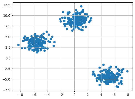
K-means clustering is a popular unsupervised machine learning algorithm used for partitioning a dataset into groups or clusters based on similarity. The algorithm aims to group data points into k clusters, where each cluster represents a set of observations that are more similar to each other than to data points in other clusters.

K-means clustering has several applications, such as customer segmentation, anomaly detection, and image compression. It is a simple and efficient algorithm, but it has some limitations. For example, it is sensitive to the initial centroid selection and can converge to different solutions depending on the starting point. It also assumes that the clusters are spherical and have equal variance.

To overcome these limitations, variations of k-means clustering have been developed, such as K-means++, which improves the initial centroid selection, and K-medoids, which uses medoids instead of centroids. Additionally, there are other clustering algorithms, such as hierarchical clustering and DBSCAN, that can be used depending on the specific requirements of the dataset and problem at hand.

Here’s an overview of how k-means clustering algorithms work:

Algorithm Steps:

• Initialization: Choose the number of clusters k. Initialize the centroids of the clusters randomly or using a predefined strategy. A centroid is a point that represents the center of a cluster.
• Assignment:  Assign each data point to the nearest centroid. This is done by measuring the Euclidean distance (or other distance metrics) between each data point and all centroids, and assigning the point to the cluster associated with the closest centroid.
• Update Centroids: Recalculate the centroids of each cluster based on the mean of the data points assigned to that cluster. The centroid becomes the new center for the cluster.
• Repeat Steps 2 and 3:  Iteratively repeat the assignment and centroid update steps until convergence or a stopping criterion is met. Convergence occurs when the assignment of data points to clusters and the positions of centroids no longer change significantly.

Objective Function:  The objective of the k-means algorithm is to minimize the sum of squared distances (within-cluster sum of squares) between data points and their assigned centroids.  Mathematically, it can be expressed as:

[latex]J=\sum_{i=1}^{k}\sum_{j=1}^{n_i}\|{x_j^{(i)}}-{c_i}{||^2}[/latex]

Where [latex]J[/latex] is the objective function, [latex]k[/latex] is the number of clusters, [latex]{n_i}[/latex] is the number of data points in cluster [latex]i[/latex], [latex]x_j^{(i)}[/latex] is the J-th data point in cluster [latex]i[/latex], and [latex]{c_i}[/latex] is the centroid of cluster [latex]i[/latex].

Determining the Number of Clusters ([latex]k[/latex]):  Selecting an appropriate value for [latex]k[/latex] is crucial.  Common methods include the elbow method, silhouette analysis, and domain knowledge to guide the choice of [latex]k[/latex].

Advantages of K-means Clustering:

• Simplicity:  K-means is straightforward and computationally efficient, making it suitable for large datasets.
• Scalability:  The algorithm scales well with the number of data points and features.
• Versatility:  K-means can be applied to a variety of data types and is not restricted to specific assumptions about the data distribution.

Limitations and Considerations:

• Sensitive to Initial Centroids:  The choice of initial centroids can impact the final clustering result, and different initializations may lead to different outcomes.
• Assumes Spherical Clusters:  K-means assumes that clusters are spherical and equally sized, which may not be appropriate for all types of data.
• Sensitive to Outliers:  Outliers or noise can influence the cluster assignments and centroids.
• Requires Predefined Number of Clusters:  The algorithm requires the user to specify the number of clusters  ([latex]k[/latex]), which may not be known in advance.
• May Converge to Local Minima: K-means can converge to local optima, and the solution depends on the initial centroids.

Despite its limitations, k-means clustering is widely used for various applications, including customer segmentation, image compression, and anomaly detection. Careful consideration of the algorithm’s assumptions and exploration of alternatives may be necessary based on the characteristics of the data.

Neural Network Algorithms

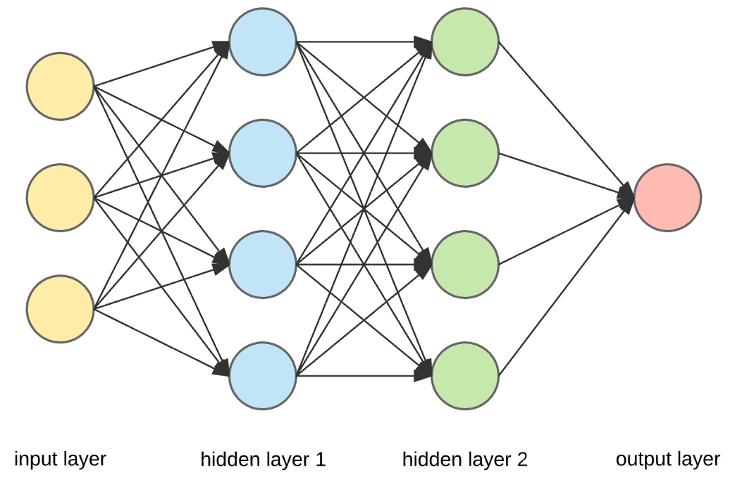
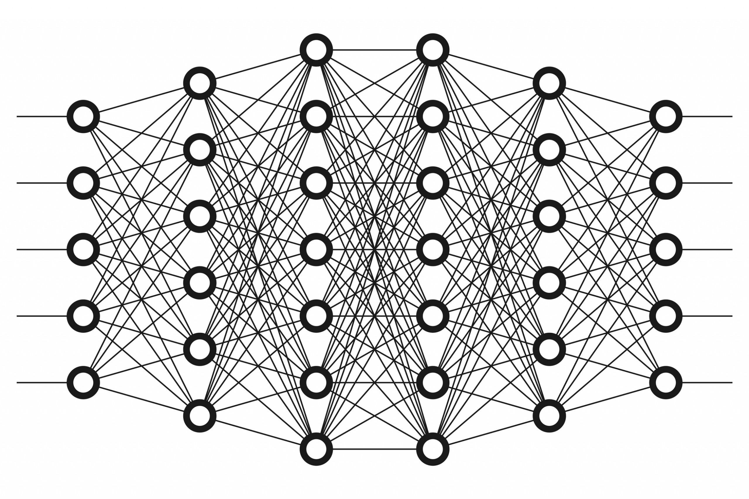
Neural networks are a class of machine learning algorithms inspired by the structure and functioning of the human brain. They are particularly powerful for tasks such as pattern recognition, classification, regression, and other complex computations. Neural networks consist of interconnected nodes (neurons) organized into layers, each layer playing a specific role in the learning process. The first layer of a neural network is called the input layer, which receives the initial data or features. The final layer is known as the output layer, which produces the desired output or prediction. In between the input and output layers, there can be one or more hidden layers, where the actual learning and computation take place.

Each neuron in a neural network receives inputs, applies a mathematical function to them, and produces an output. The outputs from one layer become the inputs for the next layer, and this process continues until the final output is generated. The mathematical function applied to the inputs is often referred to as an activation function, and it introduces non-linearity to the network, allowing it to learn complex patterns and relationships in the data.

During the learning process, neural networks adjust the weights and biases associated with each connection between neurons. This adjustment is done through a process called backpropagation, which involves propagating the error from the output layer back to the input layer and updating the weights accordingly. This iterative process of forward and backward propagation helps the network improve its predictions over time.

Neural networks have gained popularity in recent years due to their ability to handle large amounts of data and learn complex patterns. They have been successfully applied in various fields, including image and speech recognition, natural language processing, recommendation systems, and financial forecasting, among others.

However, training neural networks can be computationally expensive and requires a large amount of labeled data. Additionally, the performance of a neural network heavily depends on the architecture design, hyperparameter tuning, and the quality of the training data. Despite these challenges, neural networks continue to be a powerful tool in the field of machine learning and artificial intelligence.

Here’s a summary of how neural network algorithms work:

Basic Components of a Neural Network:

• Neurons (Nodes):  Neurons are the basic processing units in a neural network. They receive input signals, perform computations, and produce an output signal.
• Layers:  Neural networks are organized into layers, typically divided into three types:
  • Input Layer: Receives the initial input data.
  • Hidden Layers: Intermediate layers between the input and output layers, where computations and feature transformations occur.
  • Output Layer: Produces the final output or prediction.
• Weights and Biases:  Each connection between neurons has an associated weight, representing the strength of the connection. Biases are additional parameters that allow the network to adjust the output even when all inputs are zero.
• Activation Function:  The activation function introduces non-linearity to the network, enabling it to learn complex relationships in the data. Common activation functions include sigmoid, hyperbolic tangent (tanh), and rectified linear unit (ReLU).

Feedforward Process:

1. Input Propagation:  The input data is fed into the input layer. Each neuron in the input layer is connected to neurons in the first hidden layer with associated weights.
2. Hidden Layers Computation:  In each hidden layer, neurons perform a weighted sum of their inputs, add a bias, and apply the activation function. The output from each neuron becomes the input to the next layer.
3. Output Layer Computation:  The process continues through the hidden layers until the final layer (output layer) produces the network’s prediction.
4. Loss Calculation:  The difference between the predicted output and the actual target (ground truth) is quantified using a loss function. The goal is to minimize this loss during training.

Backpropagation and Training:

• Backpropagation:  Backpropagation is the process of updating the weights and biases of the network to minimize the loss. It involves calculating the gradient of the loss with respect to the weights and biases and adjusting them using optimization algorithms like stochastic gradient descent (SGD).
• Gradient Descent:  Gradient descent iteratively updates the weights and biases in the direction that minimizes the loss. This process is repeated until convergence.
• Epochs and Batches:  Training is typically performed over multiple epochs, where the entire dataset is passed through the network. In each epoch, the data is often divided into batches to enhance computational efficiency and generalization.

Model Evaluation:  Validation and Testing:  The trained model is evaluated on separate validation and testing datasets to assess its performance on unseen data and prevent overfitting.

Types of Neural Networks:

• Feedforward Neural Networks (FNN):  Traditional neural networks where information flows in one direction, from input to output. These networks consist of multiple layers of interconnected nodes, also known as neurons. Each neuron receives inputs from the previous layer and performs a series of calculations to produce an output.  The input layer of an FNN receives the initial data, which is then passed through the network’s hidden layers. Each hidden layer consists of multiple neurons that process the inputs using weighted connections. These weights determine the strength of the connections between neurons and are adjusted during the training process to optimize the network’s performance.  Finally, the processed inputs reach the output layer, where the network produces its final output. The number of neurons in the output layer depends on the specific task the FNN is designed for. For example, in a classification problem, the output layer may have neurons representing different classes, while in a regression problem, the output layer may consist of a single neuron representing a continuous value.  FNNs are trained using a process called backpropagation, which adjusts the weights in the network based on the difference between the predicted output and the desired output. This iterative process allows the network to learn from its mistakes and improve its performance over time.
• Convolutional Neural Networks (CNN):  Designed for image processing, CNNs use convolutional layers to automatically learn hierarchical features from images. Convolution preserves the spatial relationship between pixels by learning image features using small squares of input data. Each convolutional layer applies different filters like edge detection, color contrast, object detection, etc., and combines their outputs.
• Recurrent Neural Networks (RNN): Suitable for sequential data, RNNs have connections that form cycles, allowing them to capture temporal dependencies.  Unlike traditional neural networks that process input data independently without considering any previous or future information, RNNs are useful for applications such as speech recognition and time series analysis, where the order and sequence of the data is crucial for accurate prediction and understanding.  RNNs address this limitation by introducing a feedback loop in their architecture. This loop allows information to be passed from one step to the next, creating a form of memory within the network. This memory enables RNNs to retain and utilize information from previous steps when making predictions or classifications.
• Long Short-Term Memory (LSTM) and Gated Recurrent Unit (GRU): Variants of RNNs designed to overcome the limitations of traditional RNNs, such as the vanishing gradient problem and the inability to capture long-term dependencies in sequential data.  The vanishing gradient problem refers to the issue where the gradients, which are used to update the weights of the network during training, become extremely small as they propagate through time. This can result in the network being unable to effectively learn from long sequences of data. LSTM introduces a memory cell that can store information over long periods of time. It achieves this by using a combination of gates, including an input gate, a forget gate, and an output gate. These gates control the flow of information into, out of, and within the memory cell. The forget gate allows the network to selectively discard irrelevant information from the memory cell, while the input gate allows it to selectively update the cell with new information. The output gate controls the flow of information from the memory cell to the next time step.
• Autoencoders: Neural networks used for unsupervised learning and feature learning by reconstructing input data.  The basic structure of an autoencoder consists of an encoder and a decoder. The encoder takes in the input data and maps it to a compressed representation. This is then fed into the decoder, which aims to reconstruct the original input data from this compressed representation. During the training process, the autoencoder tries to minimize the reconstruction error, which is the difference between the input data and the output of the decoder. By doing so, the autoencoder learns to capture the most important features of the input data and disregard the noise or irrelevant information.  Autoencoders can be used for feature learning, where the model learns to extract meaningful features from the input data. These learned features can then be used as input for other machine learning algorithms, improving their performance.

Neural networks are highly flexible and can learn complex patterns from data, making them a foundational technology in contemporary AI and machine learning applications. The architecture, depth, and complexity of neural networks can vary based on the task at hand.

Understanding Models

In the context of ML, a model is the manifestation of an algorithm’s learning from data. It is a representation of the knowledge gained during the training phase, encapsulating the patterns, relationships, and insights derived from the input data. A model, once trained, can then make predictions or classifications on new, unseen data. The process of creating a model involves feeding a machine learning algorithm with labeled training data. The algorithm learns from this data to identify patterns and make predictions. The model’s performance is evaluated using various metrics, such as accuracy, precision, recall, and F1 score.

There are different types of models used in machine learning, depending on the problem at hand. For example, in supervised learning, the model is trained using labeled data, where each data point is associated with a target variable. The model learns to predict the target variable based on the input features.

In unsupervised learning, the model is trained on unlabeled data and aims to discover hidden patterns or structures within the data. This type of model is commonly used for tasks like clustering or dimensionality reduction.

Once a model is trained and evaluated, it can be deployed to make predictions on new, unseen data. This is called the inference phase. The model takes the input data and applies the learned patterns and relationships to make predictions or classifications.

It is important to note that models are not perfect and can have limitations. They may not generalize well to unseen data if the training data is biased or insufficient. Regular model evaluation and improvement are necessary to ensure reliable and accurate predictions.

In summary, a model in machine learning represents the knowledge gained from training data and can be used to make predictions on new data. It is the manifestation of an algorithm’s learning and encapsulates patterns, relationships, and insights derived from the input data.

Key Components:

• Parameters: The internal variables adjusted during training to optimize the model’s performance.
• Features: The input variables or attributes used by the model to make predictions.
• Output: The result or prediction generated by the model based on the input.

Training and Evaluation:

• Training Phase: The model learns from a labeled dataset, adjusting its parameters to minimize the difference between predicted and actual outcomes.
• Evaluation Phase: The model is tested on new, unseen data to assess its performance and generalizability.

Interpreting Model Output:

Interpreting the output of a model involves understanding the predictions it makes and the factors influencing those predictions. In a classification task, for example, the model assigns data points to specific categories. In regression, it predicts numerical values. The transparency and interpretability of a model are crucial considerations, especially in domains where decision-making accountability is paramount.

Considerations:

• Bias and Fairness: Models can inherit biases present in training data, raising ethical considerations.
• Generalization: A model’s ability to perform well on new, unseen data.
• Overfitting and Underfitting: Balancing model complexity to avoid memorizing noise or oversimplifying.

Understanding algorithms and models lays the foundation for effective application in diverse domains, empowering practitioners to harness the potential of ML to solve complex problems, make informed decisions, and drive innovation in the business landscape.

Supervised and Unsupervised Learning Algorithms

Supervised Learning

Supervised Learning is akin to a mentor guiding a student. In this paradigm, the algorithm is provided with a labeled dataset, where each input is paired with the corresponding desired output. The algorithm learns to map inputs to outputs by generalizing patterns from the labeled data. Think of it as a teacher supervising a learning process, correcting errors, and refining the model’s predictive capabilities.

Key Components:

• Training Data: Labeled dataset comprising input-output pairs.
• Model: The algorithm that learns patterns and relationships from the labeled data.
• Loss Function: A metric that quantifies the difference between predicted and actual outputs.
• Optimization: Adjusting the model’s parameters to minimize the loss function.

Example: In a spam email filter, the algorithm learns from labeled data (spam or not spam) to classify new emails more effectively.

Unsupervised Learning

Unsupervised Learning, in contrast, is akin to exploring a new territory without a guide. Here, the algorithm is presented with an unlabeled dataset and must uncover hidden patterns or structures within the data. The goal is not predefined; instead, the algorithm autonomously discovers meaningful insights, making it particularly useful for exploratory data analysis and clustering.

Key Components:

• Data: Unlabeled dataset without predefined outputs.
• Model: The algorithm identifies patterns, relationships, or groupings within the data.
• Objective: Discover hidden structures, reduce dimensionality, or uncover underlying relationships.

Example: In customer segmentation, an algorithm can identify distinct groups based on purchasing behavior without predefined categories.

Chapter Summary

The chapter focuses on the basic concepts of algorithms, models, and learning. It begins by explaining how linear regression can be used to predict outcomes based on a set of data. This is demonstrated by the example of predicting test scores based on study hours. The process involves four steps: data collection, finding the line of best fit through the data points, making predictions using this line, and testing the rule by comparing predicted test scores with the actual ones.

The chapter then moves on to decision-tree algorithms, likening them to choosing a path in a forest. Each decision or “node” in the tree represents a choice based on certain conditions, such as the type of tree at the start of the path. Following the signs or nodes eventually leads to a destination, demonstrating how decision trees help in making choices.

The concept of neural networks is introduced next, with an analogy of teaching a computer to recognize animals in the same way a smart 5th-grade friend does. The process involves learning from pictures, identifying features of each animal, and training the computer by showing it many pictures of animals and telling it what each animal is.

Finally, the chapter discusses the concept of finding centers in data groups. This is illustrated by using candies as data points and selecting a candy from each group that best represents the average color of the candies in its group. This process is likened to finding the center point that best represents its group.

In summary, the chapter provides a comprehensive introduction to basic concepts in algorithms and machine learning, including linear regression, decision-tree algorithms, neural networks, and finding centers in data groups. These concepts are explained using everyday analogies, making them accessible and easy to understand.